Larger Symmetries

“Further progress lies in the direction of making our equations invariant under wider and still wider transformations.”

These prophetic lines were written in 1930 by P. A. M. Dirac in his famous book “The Principles of Quantum Mechanics”. In the following centuries, tremendous progress was made exactly as he predicted.

Weak interactions were described perfectly using $SU(2)$ symmetry, strong interactions using $SU(3)$ symmetry and it is well known that electrodynamics can be derived from $U(1)$ symmetry. Other aspects of elementary particles, like their spin, can be understood using the symmetry of special relativity.

A symmetry is a transformation that leaves our equations invariant, i.e. that does not change the equations. A set of symmetry transformations is called a group and, for example, the set of transformations that leaves the equations of special relativity invariant is called the Poincare group.

By making our equations invariant under the quite large set of transformations:

$$ \text{Poincare Group} \times U(1) \times SU(2) \times SU(3) , $$

we are able to describe all known interactions of elementary particles, except for gravity. This symmetry is the core of the standard model of modern physics, which is approximately 40 years old. Since then it has been confirmed many times, for example, through the discovery of the Higgs boson. Just as Dirac predicted, we gained incredible insights into the inner workings of nature, by making the symmetry of our equations larger and larger.

Unfortunately, since the completion of the standard model $\sim 40$ years ago, there was no further progress in this direction. No further symmetry of nature was revealed by experiments. (At least that’s the standard view, but I don’t think it’s true. More on that later). In 2017 our equations are still simply invariant under $ \text{Poincare Group} \times U(1) \times SU(2) \times SU(3) , $ but no larger symmetry.

I’m a big believer in Dirac’s mantra. Despite the lack of new experimental insights, I do think there are many great ideas for how symmetries could guide us towards the correct theory beyond the standard model.

Before we can discuss some of these ideas, there is one additional thing that should be noted. Although the four groups $ \text{Poincare Group} \times U(1) \times SU(2) \times SU(3) $ are written equally next to each other, they aren’t treated equally in the standard model. The Poincare group is a spacetime symmetry, whereas all other groups describe inner symmetries of quantum fields. Therefore, we must divide the quest for a larger symmetry into two parts. On the one hand, we can enlarge the spacetime symmetry and on the other hand, we can enlarge the inner symmetry. In addition to these two approaches, we can also try to treat the symmetries equally and enlarge them at the same time.

Let’s start with the spacetime symmetry.

Enlargement of the Spacetime Symmetry

The symmetry group of special relativity is the set of transformations that describe transformations between inertial frames of reference and leave the speed of light invariant. As already noted, this set of transformations is called the Poincare group.

Before Einstein discovered special relativity, people used a spacetime symmetry that is called the Galilean group. The Galilean group also describes transformations between inertial frames of reference but does not care about the speed of light.

The effects of special relativity are only important for objects that are moving fast. For everything that moves slowly compared to the speed of light, the Galilean group is sufficient. The Galilean group is an approximate symmetry when objects move slowly. Mathematically this means that the Galilean group is the contraction of the Poincare group in the limit where the speed of light goes to infinity. For an infinite speed of light, nothing can move with a speed close to the speed of light and thus the Galilean group would be the correct symmetry group.

It is natural to wonder if the Poincare group is an approximate symmetry, too.

One hint in this direction is that the Poincare group is an “ugly” group. The Poincare group is the semi-direct product of the group of translations and the Lorentz group, which described rotations and boosts. Therefore the Poincare group, not a simple group. The simple groups are the “atoms of groups” that can be used to construct all other groups from. However, the spacetime symmetry group that we use in the standard model is not one of these truly fundamental groups.

Already in 1967, Monique Levy‐Nahas studied the question which groups could yield the Poincare group as a limit, analogous to how the Poincare group yields the Galilean group as a limit.

The answer she found was stunningly simple: “the only groups which can be contracted in the Poincaré group are $SO(4, 1)$ and $SO(3, 2)$”. These groups are called the de Sitter and the anti-de Sitter group.

They consist of transformations that describe transformations between inertial frames of reference, leave the speed of light invariant and leave additionally an energy scale invariant. The de Sitter group leaves a positive energy scale invariant, whereas the anti deSitter group leaves a negative energy scale invariant. Both contract to the Poincare group in the limit where the invariant energy scale goes to zero.

Levy‐Nahas’ discovery is great news. There isn’t some large pool of symmetries that we can choose from, but only two. In addition, the groups she found are simple groups and therefore much “prettier” than the Poincare group.

Following Dirac’s mantra and remembering the fact that the deformation: Galilean Group $\to $ Poincare Group led to incredible progress, we should take the idea of replacing the Poincare group with the de Sitter or anti de Sitter group seriously. This point was already emphasized in 1972 by Freeman J. Dyson in his famous talk “Missed opportunities”.

Nevertheless, I didn’t hear about the de Sitter groups in any particle physics lecture or read about them in any particle physics book. Maybe because the de Sitter symmetry is not a symmetry of nature? Because there is no experimental evidence?

To answer these questions, we must first answer the question: what is the energy scale that is left invariant?

The answer is: it’s the cosmological constant!

The present experimental status is that the cosmological constant is tiny but nonzero and positive: $\Lambda \approx 10^{-12}$ eV! This smallness explains why the Poincare group works so well. Nevertheless, the correct spacetime symmetry group is the de Sitter group. I’m a bit confused why this isn’t mentioned in the textbooks or lectures. If you have an idea, please let me know!

Can we enlarge the spacetime symmetry even further?

Yes, we can. But as we know from Levy‐Nahas’ paper, only a different kind of symmetry enlargement is possible. There isn’t any other symmetry that could be more exact and yield the de Sitter group in some limit. Instead, we can think about the question, if there could be a larger broken spacetime symmetry.

Nowadays the idea of a broken symmetry is well known and already an important part of the standard model. In the standard model, the Higgs field triggers the breaking $SU(2) \times U(1) \to U(1)$.

Something similar could’ve been happened to a spacetime symmetry in the early universe. A good candidate for such a broken spacetime symmetry is the conformal group $SO(4,2)$.

The temperature in the early universe was incredibly high and “[i]t is an old idea in particle physics that, in some sense, at sufficiently high energies the masses of the elementary particles should become unimportant” (Sidney Coleman in Aspects of Symmetry). In the massless limit, our equations become invariant under the conformal group (source). The de Sitter group and the Poincare group are subgroups of the conformal group. Therefore it is possible that the conformal group was broken to the de Sitter group in the early universe.

This idea is interesting for a different reason, too. The only parameter in the standard model that breaks conformal symmetry at tree level is the Higgs mass parameter. This parameter is the most problematic aspect of the standard model and possibly the Higgs mass fine-tuning problem can be solved with the help of the conformal group. (See: On naturalness in the standard model by William A. Bardeen.)

Enlargement of the Inner Symmetry

The inner symmetry group of the standard model $ U(1) \times SU(2) \times SU(3) $ is quite ugly, too. Like the Poincare group, it is not a simple group.

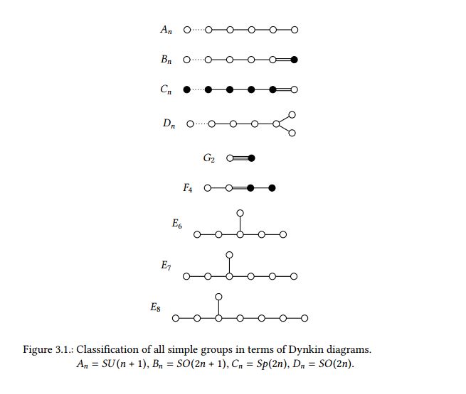
There is an old idea by Howard Georgi and Sheldon Glashow that instead of $ U(1) \times SU(2) \times SU(3) $ we use a larger, simple group $G_{GUT} $. These kinds of theories are called Grand Unified Theories (GUTs).

While GUTs have problems, they are certainly beautiful. On obvious “problem” is that in present-day colliders, we do not observe effects of a $G_{GUT}$ structure and thus we assume the unified gauge symmetry is broken at some high energy scale:

\begin{equation} \label{eq:schematicgutbreaking}
G_{GUT} \stackrel{M_{GUT}}{\rightarrow} \ldots \stackrel{M_I}{\rightarrow} G_{SM} \stackrel{M_Z}{\rightarrow} SU(3)_C \times U(1)_Q \, ,
\end{equation}

where the dots indicate possible intermediate scales between $G_{GUT}$ and $G_{SM}$. In the following, we discuss some of the “mysteries” of the standard model that can be resolved by a GUT.

Quantization of Electric Charge

In the standard model the electric charges of the various particles must be put in by hand and there is no reason why there should be any relation between the electron and proton charge. However from experiments it is known that $Q_{\text{proton}}+Q_{\text{electron}}= \mathcal{O}(10^{-20})$. In GUTs one multiplet of $G_{GUT}$ contains quarks and leptons. This way, GUTs provide an elegant explanation for the experimental fact of charge quantization. For example in $SU(5)$ GUTs the conjugate $5$-dimensional representation contains the down quark and the lepton doublet

\begin{equation}
\bar{5} = \begin{pmatrix} \nu_L \\ e_L \\ (d_R^c)_{\text{red}} \\ (d_R^c)_{\text{blue}} \, .\\ (d_R^c)_{\text{green}} \end{pmatrix}
\end{equation}

The standard model generators must correspond to generators of $G_{GUT}$. Thus the electric charge generator must correspond to one Cartan generator of $G_{GUT}$ (The eigenvalues of the Cartan generators of a given gauge group correspond to the quantum numbers commonly used in particle physics.). In $SU(5)$ the Cartan generators can be written as diagonal $5\times 5$ matrices with trace zero. (In $SU(5)$ is the set of $5 \times 5$ matrices $U$ with determinant $1$ that fulfil $U^\dagger U = 1$. For the generators $T_a$ this means $\text{det}(e^{i \alpha_a T_a})=e^{i \alpha_a \text{Tr}(T_a)} \stackrel{!}{=}1$. Therefore $Tr(T_a) \stackrel{!}{=} 0$) Therefore we have

\begin{align}
\text{Tr}(Q)&= \text{Tr} \begin{pmatrix} Q(\nu_L) & 0 & 0 & 0 &0 \\ 0 & Q(e_L) & 0 & 0 &0 \\ 0 & 0 & Q((d_R^c)_{\text{red}}) & 0 &0\\ 0 & 0 & 0 & Q((d_R^c)_{\text{blue}})&0\\ 0 & 0 & 0 & 0 &Q((d_R^c)_{\text{green}}) \end{pmatrix} \stackrel{!}{=} 0 \notag \\
&\rightarrow Q(\nu_L) + Q(e_L) + 3Q(d_R^c) \stackrel{!}{=} 0 \notag \\
&\rightarrow Q(d_R^c) \stackrel{!}{=} -\frac{1}{3} Q(e_L) \, .
\end{align}

Analogously, we can derive a relation between $e_R^c$, $u_L$ and $u_R^c$. Thus $Q_{\text{proton}}+Q_{\text{electron}}= \mathcal{O}(10^{-20})$ is no longer a miracle, but rather a direct consequence of of the embedding of $G_{SM}$ in an enlarged gauge symmetry.

Coupling Strengths

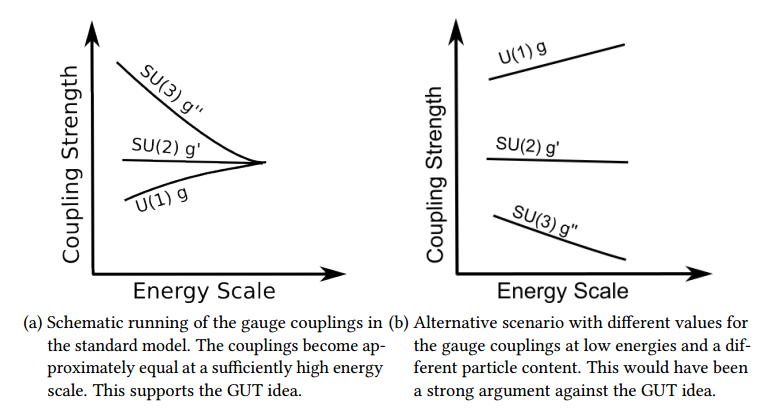
The standard model contains three gauge couplings, which are very different in strength. Again, this is not a real problem of the standard model, because we can simply put these values in by hand. However, GUTs provide a beautiful explanation for this difference in strength. A simple group $G_{GUT}$ implies that we have only one gauge coupling as long as $G_{GUT}$ is unbroken. The gauge symmetry $G_{GUT}$ is broken at some high energy scale in the early universe. Afterward, we have three distinct gauge couplings with approximately equal strength. The gauge couplings are not constant but depend on the energy scale. This is described by the renormalization group equations (RGEs). The RGEs for a gauge coupling depends on the number of particles that carry the corresponding charge. Gauge bosons have the effect that a given gauge coupling becomes stronger at lower energies and fermions have the opposite effect. The adjoint of $SU(3)$ is $8$-dimensional and therefore we have $8$ corresponding gauge bosons. In contrast, the adjoint of $SU(2)$ is $3$-dimensional and thus we have $3$ gauge bosons. For $U(1)$ there is only one gauge boson. As a result for $SU(3)$ the gauge boson effect dominates and the corresponding gauge coupling becomes stronger at lower energies. For $SU(2)$ the fermion and boson effect almost cancel each other and thus the corresponding gauge coupling is approximately constant. For $U(1)$ the fermions dominate and the $U(1)$ gauge coupling becomes much weaker at low energies. This is shown schematically in the figure below. This way GUTs provide an explanation why strong interactions are strong and weak interactions are weak.


Another interesting aspect of the renormalization group evolution of the gauge couplings is that there is a close between the GUT scale and the proton lifetime. Thus proton decay experiments yield directly a bound on the GUT scale $M_{GUT} \gtrsim
10^{15}$ GeV. On the other hand, we can use the measured values of the gauge couplings and the standard model particle content to calculate how the three standard model gauge couplings change with energy. Thus we can approximate the GUT scale as the energy scale at which the couplings become approximately equal. The exact scale depends on the details of the GUT model, but the general result is a very high scale, which is surprisingly close to the value from proton decay experiments. This is not a foregone conclusion. With a different particle content or different measured values of the gauge coupling, this calculation could yield a much lower scale and this would be a strong argument against GUTs. In addition, the gauge couplings could run in the “wrong direction” as shown in the figure. The fact that the gauge coupling run sufficiently slow and become approximately equal at high energies are therefore hints in favor of the GUT idea.


Further Postdictions

In addition to the “classical” GUT postdictions described in the last two sections, I want to mention two additional postdictions:

  • A quite generic implication of grand unification small neutrino masses through the type-1 seesaw mechanism. Models based on the popular $SO(10)$ or $E_6$ groups contain automatically a right-handed neutrino $\nu_R$. As a result of the breaking chain this standard model singlet $\nu_R$ gets a superheavy mass $M$. After the last breaking step $G_{SM}\rightarrow SU(3)_C \times U(1)_Y$ the right-handed and left-handed neutrinos mix. This yields a suppressed mass of the left-handed neutrino of order $\frac{m^2}{M}$, where $m$ denotes a typical standard model mass.
  •  GUTs provide a natural framework to explain the observed matter-antimatter asymmetry in the universe. As already noted above a general implication of GUTs is that protons are no longer stable. Formulated differently, GUTs allow baryon number-violating interactions. This is one of three central ingredients, known as Sakharov condition, needed to produce more baryons than antibaryons in the early universe. Thus, as D. V. Nanopoulos put it, “if the proton was stable it would not exist”.


What’s next?


While the unification of spacetime symmetries was already confirmed by the measurement of the cosmological constant, so far, there is no experimental evidence for the correctness of the GUT idea. Thus the unification of internal symmetries still has to wait. However, proton decay could be detected anytime soon. When Hyper-Kamiokande will start operating the limits on proton lifetime will become one order of magnitude better and this means there is a realistic chance that we finally find evidence for Grand Unification.

This, however, would by no means be the end of the road.

Arguably, it would be awesome if we could unify spacetime and internal symmetries into one large symmetry. However, there is one no-go theorem that blocked progress in this direction: the famous Coleman-Mandula theorem.

Nevertheless, a no-go theorem in physics never really means that something is impossible, only that it isn’t as trivial as one might think. There are several loopholes in the theorem, that potentially allow the unification of spacetime and internal symmetries.

At least to m, it seems as Dirac was right and larger symmetries is the way to go. However, so far, we don’t know which way we should follow.

What are Quantum Numbers?

For quite some time I didn’t really understand what quantum numbers are. For example, why do we use the words “red”, “blue” and “green” for the charges of the strong interaction? Why does a gluon carry “red anti-green + green anti-red” color? From the group theoretical perspective these things actually make a lot of sense and maybe this post helps someone who is equally confused as I was a few years ago.

First, we recall that a Lie algebra representation is a map $R$ from the Lie algebra $\mathfrak{g}$ of a group $G$ to the linear operators $\mathrm{Lin}(\cdot)$ over some vector space $V$.
\begin{equation}
R: \ \mathfrak{g}  \rightarrow \mathrm{Lin}(V) \, .
\end{equation}

The easiest example is the fundamental $2$-dimensional representation of $\mathfrak{su}(2)$, which is a map

\begin{equation}
R: \ \mathfrak{su}(2)  \rightarrow \mathrm{Lin}(\mathbb{C}^2) \, .
\end{equation}

In words this means that this representation maps each element of $\mathfrak{su}(2)$ onto a $2 \times 2$ matrix that acts on $2$-dimensional vectors. A basis for this Lie algebra is given by

\begin{align}
T_1&=\frac{1}{2} \sigma_1 =  \frac{1}{2} \begin{pmatrix} 0 & 1 \\ 1 & 0 \end{pmatrix} \, , \notag \\
T_2&=\frac{1}{2} \sigma_2 =  \frac{1}{2} \begin{pmatrix} 0 & -\mathrm{i} \\ \mathrm{i} & 0 \end{pmatrix} \, , \notag  \\
T_3&=\frac{1}{2} \sigma_3 =  \frac{1}{2} \begin{pmatrix} 1 & 0 \\ 0 & -1 \end{pmatrix} \, ,
\end{align}

where $\sigma_i$ denote the usual Pauli matrices.

From linear algebra we know that the eigenvectors of a linear operator always form a basis for the vector space in question. In addition, for any Lie group, one or more of the generators can be simultaneously diagonalized using similarity transformations. The set of generators that can be diagonalized simultaneously are called Cartan generators. Thus, a suggestive and particularly easy basis for the vector space of each representation is given by the eigenvectors of the Cartan generators. An easy way to label these basis vectors is to use the corresponding eigenvalues.

In particle physics the fundamental particles are (among others) labelled by their color and weak-isospin. These quantum numbers correspond to eigenvalues of the Cartan generators of the corresponding gauge groups. For $SU(2)_L$, the gauge group of weak-interactions, there is only one Cartan generator and in the fundamental two-dimensional representation it is given by

\begin{equation}
I_3 = \frac{1}{2} \sigma_3 = \frac{1}{2} \begin{pmatrix} 1 & 0 \\ 0 & -1 \end{pmatrix} \, .
\end{equation}

The factor $\frac{1}{2} $ is there, because we usually normalize our generators such that the Dynkin index Tr$(T_a T_a)$ for this generator in the fundamental representation of the Lie algebra is $\frac{1}{2}$.

The corresponding eigenvalues are $\frac{1}{2}$ and $-\frac{1}{2}$. This means particles that correspond to $SU(2)_L$ eigenstates in the fundamental $2$-dimensional representation are with respect to $SU(2)_L$

\begin{equation}
\begin{pmatrix} 1 \\ 0 \end{pmatrix} \ \text{ with isospin } \frac{1}{2} \quad , \quad \begin{pmatrix} 0 \\ 1 \end{pmatrix} \ \text{ with isospin } -\frac{1}{2} \, .
\end{equation}

Less trivial is $SU(3)$, the gauge group of strong interactions, because there are two Cartan generators. In the representation that acts on the fundamental $3$-dimensional representation they can be written as

\begin{equation} \label{eq:cartansu3}
H_1=
\frac{1}{2} \left( \begin{array}{ccc}
1 & 0 & 0 \\
0 & 0 & 0 \\
0 & 0 & -1
\end{array} \right) \quad , \quad H_2 = \frac{1}{2 \sqrt{3}} \left( \begin{array}{ccc}
1 & 0 & 0 \\
0 & -2 & 0 \\
0 & 0 & 1
\end{array} \right) \, .
\end{equation}

Again, we label the trivial eigenvectors using the the eigenvalues of the Cartan generators. However, now there are two eigenvalues for each eigenvector and therefore we define objects, called weights, that collect these numbers for each eigenvector. This means the $SU(3)_C$ quantum numbers for the basis vectors of the fundamental $3$-dimensional representation are

\begin{equation}
\left(\frac{1}{2} , \frac{1}{2 \sqrt{3}} \right) \mathrm{ \ for \ }  \begin{pmatrix}
1 \\ 0 \\ 0
\end{pmatrix} \quad , \quad \left(0 , \frac{-1}{ \sqrt{3}} \right) \mathrm{ \ for \ }  \begin{pmatrix}
0 \\ 1 \\ 0
\end{pmatrix}  \quad , \quad \left(-\frac{1}{2} , \frac{1}{2 \sqrt{3}} \right) \mathrm{ \ for \ }  \begin{pmatrix}
0 \\ 0 \\ 1
\end{pmatrix}  \,  .
\end{equation}

It is conventional to replaces these weights with names: red $:=(\frac{1}{2} , \frac{1}{2 \sqrt{3}})$, blue $:=(0 , \frac{-1}{ \sqrt{3}})$, green $:=(\frac{-1}{2} , \frac{1}{2 \sqrt{3}})$. The labels for the conjugate fundamental representation $\bar 3$ are simply minus the labels of the fundamental $3$ and are called anti-red, anti-blue and anti-green.

We can use these basis vectors and the corresponding weights to derive the basis vectors and weights for product representations like

\begin{equation} \label{eq:3x3bardecomposition}
3 \otimes \bar 3 = 1 \oplus 8 \, .
\end{equation}

The $8$ is the adjoint representation of $SU(3)$ and Eq. \ref{eq:3x3bardecomposition} tells us that we can write each element of the adjoint as $3\times 3$ matrix. For the basis vectors we use

\begin{equation}
e_{ij} = e_i \otimes e_j \, .
\end{equation}

For the quantum numbers of the product representations we use

\begin{equation}
QN \big ( (a \otimes b)_{ij} \big) = QN(a_i) + QN( b_j) \, .
\end{equation}

Formulated in terms of weights this means that we can compute the weight corresponding to the $ij$ element of the product representation $3 \otimes \bar{3}=1 \oplus 8$ by adding the weights of $3_i$ and $\bar{3}_j$

\begin{equation}
w\Big ( (3 \otimes 3)_{ij}\Big) = w(3_i) + w(3_j) \,.
\end{equation}

The $3 \times 3$ matrix that correspond to this weights is given by the Kronecker product of the $i$-th and $j$-th basis vector. Thus we have

\begin{equation}
\left(
\begin{array}{cc}
\frac{1}{2} & \frac{\sqrt{3}}{2} \\
\end{array}
\right) = \left( \begin{array}{ccc}
0 & 1 & 0 \\
0 & 0 & 0 \\
0 & 0 & 0
\end{array} \right) \, , \quad  \left(
\begin{array}{cc}
1 & 0 \\
\end{array}
\right)=  \left( \begin{array}{ccc}
0 & 0 & 1 \\
0 & 0 & 0 \\
0 & 0 & 0
\end{array} \right) \, , \quad \left(
\begin{array}{cc}
\frac{1}{2} & -\frac{\sqrt{3}}{2} \\
\end{array}
\right) = \left( \begin{array}{ccc}
0 & 0 & 0 \\
0 & 0 & 1 \\
0 & 0 & 0
\end{array} \right) \, , \end{equation} \begin{equation}  \left(
\begin{array}{cc}
-\frac{1}{2} & -\frac{\sqrt{3}}{2} \\
\end{array}
\right)=
\left( \begin{array}{ccc}
0 & 0 & 0 \\
1 & 0 & 0 \\
0 & 0 & 0
\end{array} \right) \, , \quad \left(
\begin{array}{cc}
-1 & 0 \\
\end{array}
\right) = \left( \begin{array}{ccc}
0 & 0 & 0 \\
0 & 0 & 0 \\
1 & 0 & 0
\end{array} \right) \, , \quad \left(
\begin{array}{cc}
-\frac{1}{2} & \frac{\sqrt{3}}{2}
\end{array}
\right) = \left( \begin{array}{ccc}
0 & 0 & 0 \\
0 & 0 & 0 \\
0 & 1 & 0
\end{array} \right) \,
\end{equation}

and two zero weights $(0,0)$ that span a basis for the Cartan subalgebra

\begin{equation} \left(
\begin{array}{cc}
0 &0\\
\end{array}
\right)_1=  \frac{1}{2} \left( \begin{array}{ccc}
1 & 0 & 0 \\
0 & 0 & 0 \\
0 & 0 & -1
\end{array} \right)  \, , \quad   \left(
\begin{array}{cc}
0 & 0 \\
\end{array}
\right)_2 =  \frac{1}{2 \sqrt{3}} \left( \begin{array}{ccc}
1 & 0 & 0 \\
0 & -2 & 0 \\
0 & 0 & 1
\end{array} \right) \, .
\end{equation}

These $8$ matrices are given in a basis, known as Cartan-Weyl basis for $\mathfrak{su}(3) $. The special thing about this basis is that each matrix here is an “eigenmatrix” of the Cartan generators $H_i$, which means

\begin{equation}
H_i \circ M = [H_i,M]=\lambda_i M \, ,
\end{equation}

where $\lambda_i$ is the eigenvalue for the Cartan generator $H_i$. In physical terms, each of these $8$ matrices represents a different gluon. This is completely analogous to how the three basis vectors for $\mathbb{R}^3$ for the fundamental representation correspond to three different quarks: a red quark, a blue quark and a green quark.

There is another way to denote gluons, analogous to the color notation for quarks in the fundamental $3$. We can use the fact that each gluon corresponds to a product of a basis vector of the fundamental $3$ and basis vector of the anti-fundamental $\bar{3}$, to name each gluon in terms of color, too. For example, for $i=1$ and $j=2$

\begin{equation}
8_{12} \hat= w(3_1) + w( \bar{3}_2)  = \left(\frac{1}{2} , \frac{1}{2 \sqrt{3}} \right) +\left(0 , \frac{1}{ \sqrt{3}}\right) = \text{red+ anti-blue} =\left( \frac{1}{2},  \frac{\sqrt{3}}{2} \right)  \, .
\end{equation}

Therefore just as we have red, blue and green quarks, we have $8$ gluons that we can label by color combinations of the form color-anticolor.

There is another basis for the $8$ basis matrices of the adjoint representation, more popular among physicists, called the Gell-Mann basis\footnote{The Gell-Mann basis is more popular due to the close connection to the Pauli matrices of $SU(2)$.}. In this basis the $8$ basis elements $T_a$ of $\mathfrak{su}(3) $ are given in terms of the $8$ Gell-Mann matrices $\lambda_a$ by $T_a= \frac{1}{2} \lambda_a$, where
\begin{equation}\label{lambda1-3}
\lambda_1 =
\begin{array}{ccc}
\left(
\begin{array}{ccc}
0 & 1 & 0 \\
1 & 0 & 0 \\
0 & 0 & 0
\end{array}
\right),
&
\lambda_2 =\left(
\begin{array}{ccc}
0 & -i & 0 \\
i & 0 & 0 \\
0 & 0 & 0
\end{array}
\right),
&
\lambda_3 =\left(
\begin{array}{ccc}
1 & 0 & 0 \\
0 & 0 & 0 \\
0 & 0 & -1
\end{array}
\right),
\end{array}
\end{equation}

\begin{equation}\label{lamdba4-6}
\begin{array}{ccc}
\lambda_4 =\left(
\begin{array}{ccc}
0 & 0 & 1 \\
0 & 0 & 0 \\
1 & 0 & 0
\end{array}
\right),
&
\lambda_5 =\left(
\begin{array}{ccc}
0 & 0 & i \\
0 & 0 & 0 \\
-i & 0 & 0
\end{array}
\right),
&\lambda_6 =\left(
\begin{array}{ccc}
0 & 0 & 0 \\
0 & 0 & 1 \\
0 & 1 & 0
\end{array}
\right),
\end{array}
\end{equation}

\begin{equation}\label{lambda7-8}
\begin{array}{cc}
\lambda_7 =\left(
\begin{array}{ccc}
0 & 0 & 0 \\
0 & 0 & -i \\
0 & i & 0
\end{array}
\right),
&
\lambda_8=\frac{1}{\sqrt{3}}\left(
\begin{array}{ccc}
1 & 0 & 0 \\
0 & -2 & 0 \\
0 & 0 & 1
\end{array}
\right).
\end{array}
\end{equation}

Again, we can give names in the form color-anticolor to the gluon states in this basis. For example,

\begin{align}
T_1 &= \frac{1}{2}\lambda_1 =
\left(
\begin{array}{ccc}
0 & 1 & 0 \\
1 & 0 & 0 \\
0 & 0 & 0
\end{array}
\right)
= \left(
\begin{array}{ccc}
0 & 1 & 0 \\
0 & 0 & 0 \\
0 & 0 & 0
\end{array}
\right) + \left(
\begin{array}{ccc}
0 &0 & 0 \\
1 & 0 & 0 \\
0 & 0 & 0
\end{array}
\right)  \notag \\ &= \text{red anti-green} + \text{green anti-red}
\end{align}

and this is a popular way to label the gluons.

Classification of all Simple Lie Groups

Simple Lie groups are important, because they are in some sense the building block we can use to build up all Lie groups. Or formulated differently: simple Lie groups are the atoms of Lie theory. They are especially important in theories that unify the fundamental forces, because of the gauge group of the theory is a simple Lie group we only have one coupling constant. In contrast, the standard model gauge group $SU(3) \times SU(2) \times U(1)$ is a product of three simple groups and hence we have three different coupling constants, i.e. three different fundamental interactions.

All simple Lie groups can be classified in terms of four infinite series $SU(n+1),SO(2n),SO(2n+1),Sp(2n)$ with $n\ge 1$, and five exceptional groups $G_2,F_4,E_6,E_7,E_8$.

In order to understand this classification it is instructive to use an algebraic approach to group theory. One way to define simple Lie algebras is as antihermitian matrices, which are closed under Lie bracket multiplication and fulfill the Jacobi identity
\begin{equation} \label{eq:jacobiidentity}
[[X,Y],Z]+[[Y,Z],X]+[[Z,X],Y]=0 \, .
\end{equation}

The generators of $SO(n)$ are given by antihermitian matrices with trace zero and real numbers as matrix entries. Analogously the generators of $SU(n)$ are given by antihermitian matrices with trace zero and complex numbers as matrix entries. If we now want to search for additional simple Lie groups beyond $SO(n)$ and $SU(n)$, we need to ask if there are generalized version of the complex numbers. One such generalization was found by W. Hamilton, surprisingly not with two complex units, but with three complex units $\mathrm{i},\mathrm{j}$ and $\mathrm{k}$. These four-dimensional complex numbers are called quaternions $\mathbb{H}$ and can be written as

\begin{equation}
q = a_1 + a_2 \mathrm{i} +a_3 \mathrm{j} + a_4 \mathrm{k} \,
\end{equation}

where
\begin{equation}
\mathrm{i}^2=\mathrm{j}^2=\mathrm{k}^2=-1 \text{ and  } \mathrm{ijk} = -1 \quad \text{and} \quad a_1,a_2,a_3,a_4 \in \mathbb{R} \, .
\end{equation}

One curious feature of quaternions it that they do not commute $q_1 q_2 \neq q_2 q_1 $. Coming back to Lie groups, there is indeed a family of simple Lie groups given by antihermitian matrices with quaternions as matrix entries. However due to the non-commutative nature of the quaternions these generators no longer have trace zero. This family of Lie groups is known as the symplectic groups $Sp(n)$. To summarize

\begin{align}
\mathfrak{so}(n) &= \{ x \in \mathbb{R}[n]: x^\dagger = -x, \text{tr}(x)=0\} \, \notag ,\\
\mathfrak{su}(n) &= \{ x \in \mathbb{C}[n]: x^\dagger = -x, \text{tr}(x)=0\} \, \notag ,\\
\mathfrak{sp}(n) &= \{ x \in \mathbb{H}[n]: x^\dagger = -x \} \, .
\end{align}

It turns out there is exactly one additional higher-dimensional version of the complex numbers, called octonions $\mathbb{O}$, with seven complex units. These were discovered shortly after the quaternions by J. Graves. Octonions are neither commutative nor associative, i.e. $(o_1 o_2) o_3 \neq o_1 (o_2 o_3)$. Due to this curious feature, octonions can not be represented by matrices, because the matrix product is associative.

In contrast, the complex numbers, can be represented by real $2\times 2$ matrices using
\begin{equation} \label{eq:comrealmatrix} 1 \mapsto
\begin{pmatrix}
1&0 \\ 0&1
\end{pmatrix}
\qquad , \qquad
\mathrm{i} \mapsto
\begin{pmatrix}
0&-1 \\ 1&0
\end{pmatrix} \, , \notag \end{equation}
which fulfil
\begin{equation} 1^2=1, \qquad \qquad \mathrm{i}^2=-1, \qquad \qquad 1\mathrm{i}=\mathrm{i}1=\mathrm{i} .\notag \end{equation}

Analogously quaternions can be written as complex $2 \times 2$ matrices, using
\begin{equation}
\mathrm{1} \mapsto
\begin{pmatrix}
1&0 \\ 0&1
\end{pmatrix}
\quad , \quad \mathrm{i} \mapsto
\begin{pmatrix}
i&0 \\ 0&-i
\end{pmatrix} \quad , \quad \mathrm{j} \mapsto
\begin{pmatrix}
0&1 \\ -1&0
\end{pmatrix}
\quad , \quad
\mathrm{k} \mapsto
\begin{pmatrix}
0&i\\i&0
\end{pmatrix} \, \notag .
\end{equation}

In abstract terms $\mathbb{R},\mathbb{C},\mathbb{H}$ and $\mathbb{O}$ are called normed division algebras, which are defined by

\begin{align}
ab&=0 \text{  only for  } a= 0 \text{  or  } b=0 \, , \notag \\
N(ab)&= N(a)N(b) \, ,
\end{align}

where $a$ and be $b$ denote arbitrary elements of the algebra and $N(\cdot)$ the associated norm. It was proven by Hurwitz that the only normed division algebras are $\mathbb{R},\mathbb{C},\mathbb{H}$ and $\mathbb{O}$. For this reason normed division algebras are sometimes called Hurwitz algebras.

With this knowledge it is natural to ask if we can find, analogous to $SO(n)$ for $\mathbb{R}$, $SU(n)$ for $\mathbb{C}$ or $Sp(n)$ for $\mathbb{H}$, a family of simple Lie groups related to the octonions. Although antihermitian matrices over octonions close under the Lie bracket they do not necessarily generate Lie groups, because of the Jacobi identity (Eq. \ref{eq:jacobiidentity}). For antihermitian matrices over the reals, complexes or quaternions this requirement is automatically satisfied due to associativity. The octonions, however, are non-associative. Therefore we need more sophisticated techniques to construct Lie algebras from octonions. It turns out there are exactly five Lie algebras one can construct using octonions, called $G_2,F_4,E_6,E_7$ and $E_8$, and not infinitely many as for the reals, complexes or quaternions. The reasons is that for four of these the explicit construction the Lie algebra involves two of the normed division algebras and there are only four distinct pairs involving the octonions

  • $(\mathbb{R},\mathbb{O})$ : $F_4$
  • $(\mathbb{C},\mathbb{O})$ : $E_6$
  • $(\mathbb{H},\mathbb{O})$ : $E_7$
  • $(\mathbb{O},\mathbb{O})$ : $E_8$

Analogously one can pair all other normed division algebras, but these yield no new Lie algebras. For example, the same construction for $(\mathbb{C},\mathbb{H})$ yields $SO(12)$. The complete set of Lie algebras one gets from this construction of composition Lie algebras is usually arranged in a square, famously known as the Freudenthal magic square.

The explicit construction of these Lie algebras would lead us too far apart from the main theme of this thesis, but can be found, for example, in this paper by Pierre Ramond. The fifth exceptional group $G_2$, is the automorphism group of the octonions. This means this group is given by the set of transformations that maps the octonions onto themselves.

To summarize, all simple Lie groups can be classified because there is a close connection to normed division algebras. Hurwitz’s theorem tells us that there are only four normed division algebras $\mathbb{R},\mathbb{C},\mathbb{H}$ and $\mathbb{O}$. Each of them is closely connected to a family of simple Lie groups, $SO(n)$, $SU(n)$, $Sp(n)$ and the exceptional groups, respectively. The construction of the corresponding generators is straightforward for the infinite families $SO(n)$, $SU(n)$, $Sp(n)$, but due to the non-associative nature of the octonions quite involved for the exceptional groups. An important result is that for this reason the exceptional family has only five members $G_2,F_4,E_6,E_7$ and $E_8$.

This classification of the simple Lie groups can be nicely summarized visualized in in terms of Dynkin diagrams as shown in the following figure.

dynkinclassification