The perturbation series in QFT is an “invention of the devil” and this is actually a good thing

In quantum field theory, we can’t calculate things exactly but instead must use a perturbative approach. This means, we calculate observables in terms of a perturbative series: $\mathcal{O}= \sum_n c_n \alpha^n$.

This approach works amazingly well. The most famous example is the magnetic dipole moment of the electron $a_e \equiv (g – 2)/2$. It was calculated to order $\alpha^5$ in Phys. Rev. Lett. 109, 111807 and this result agrees perfectly with the measured value:

$$a_e(exp) – a_e(theory) = −1.06 \ (0.82) \times 10^{-12}$$

However, there is one thing that seems to cast a dark shadow over this rosy picture: there are good reasons to believe that if we would sum up all the terms in the perturbative series, we wouldn’t get a perfectly accurate result, but instead infinity: $ \sum_n^\infty c_n \alpha^n = \infty$. This is not some esoteric thought but widely believed among experts. For example,

The only difficulty is that these expansions will at best be asymptotic expansions only; there is no reason to expect a finite radius of convergence.

G. ‘t Hooft, “Quantum Field Theory for Elementary Particles. Is quantum field theory a theory?”, 1984

Quantum field theoretic divergences arise in several ways. First of all, there is the lack of convergence of the perturbation series, which at best is an asymptotic series.

R. Jackiw, “The Unreasonable Effectiveness of Quantum Field Theory”, 1996


It has been known for a long time that the perturbation expansions in QED and QCD, after renormalization, are not convergent series.

G. Altarelli, “Introduction to Renormalons”, 1995

And this is really just a small sample of people you could quote.

This is puzzling, because as is “well known”:

Divergent series are the invention of the devil, and it is shameful to base on them any demonstration whatsoever.

Niels Hendrik Abel, 1828

In this sense, the perturbation series in QFT is an “invention of the devil” and we need to wonder $ \sum_n^\infty c_n \alpha^n = \infty \quad \Rightarrow $ ???

But, of course, before we deal with that, we need to talk about why this divergence of the perturbation series is so widely believed.

Does the perturbation series converge?

$$\mathcal{O}(\alpha)= c_0 + \alpha c_1 + \alpha^2 c_2 + \ldots $$

To answer this question, Dyson already in 1952 published a paper titled “Divergence of perturbation theory in quantum electrodynamics” in which he put forward the clever idea to exploit one of the basic theorems of analysis.

The theorem is: If $0 < r < \infty$, the series converges absolutely for every real number $\alpha$ such that $|\alpha|<r$ and diverges outside of this radius. Here, $r$ is called the radius of convergence and is a non-negative real number or $\infty$ such that the series converges if $|\alpha| < r$.

The important subtlety implied by this theorem that Dyson focused on is that if the radius of convergence is finite $\neq 0$, according to the theorem, the series would also converge for small negative $\alpha$.

In other words: If a series converges it always converges on a disk!

Dyson idea to answer the question “Does the perturbation series converge?” is that we should check if the theory makes sense for a negative value of the coupling constant $\alpha$. If we can argue somehow that the theory explodes for any negative $\alpha$ then we know immediately that $r =0$ and therefore that the perturbation series diverges.

Does QED make sense with negative $\alpha$?

Before we discuss Dyson’s argument why the theory explodes for negative $\alpha$ in detail, here is a short summary of the main line of thought:

We consider a “fictitious world” with negative $\alpha$. In such a world, equal charges attract each other, and opposite charges repel each other.

With some further thought, we will discuss in a moment, this means that the energy is no longer bounded from below. Therefore, in a world with negative $\alpha$, there is no stable ground state.

For our perturbation series, this means, that it is non-analytic around $\alpha = 0$. In other words, electrodynamics with negative $\alpha$, cannot be described by well-defined analytic functions. Therefore we can conclude that the radius of convergence is zero $r=0$, which implies that the perturbation series in QFT diverges also for a positive value of $\alpha$.

In other words, the physics as soon as $\alpha$ becomes negative is so dramatically different that we expect a singularity at $\alpha =0$. Consequently, there doesn’t exist a convergent perturbation series.

After this short summary, let’s discuss how this comes about in more detail.

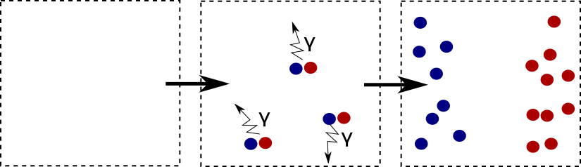
The important change as soon as $\alpha$ becomes negative is that equal charges start to attract each other. In the “normal” world with positive $\alpha$ a pair of, say, electron and positron that are created from the vacuum attract each other and therefore annihilate immediately, In a world with negative $\alpha$ they repel each other and therefore fly away from each other instead of annihilating.

This means, the naive empty vacuum state starts to fill up with electrons and positrons when $\alpha$ is negative.

Wait, is this energetically possible? What’s the energy of this new state full of electrons and positrons?

To answer this question, let’s consider a ball with radius $R$ full of electrons and calculate its energy content.

On the one hand, we have the positive rest + kinetic energy, which are proportional to the number of particles inside the ball $\propto N$.

On the other hand, we have the negative potential energy, which is given by the usual formula for a Coulomb potential $\propto N^2 R^{-1}$.

To compare them with each other, we need to know the number of electrons inside the ball. According to the Pauli principle, this number is proportional to the volume of the ball and therefore we conclude $\propto V \propto R^3 \propto N$.

Therefore, the positive part of the energy is proportional to $R^3$, and the negative energy to $\propto N^2 R^{-1} \propto R^5$. The negative part wins.

The total energy of the electrons inside the ball is negative. Most disturbingly the energy is unbounded from below and becomes arbitrarily negative as we make the ball bigger: $R,N \to \infty$.

Take note that this is only the case in our fictitious world with negative $\alpha$. In our normal world with positive $\alpha$, opposite charges attract each other and this repulsion sets a lower bound on the energy. The analogous situation to the ball above in our fictitious world is a ball full of electron-positron pairs.

The crucial thing is now that we can’t lower the energy indefinitely because when we try to group more and more electron-positron pairs together, we necessarily bring electrons close to other electrons and positrons close to other positrons. These equal charged particles repel each other in our normal world and this sets a lower bound on the energy.

So, to conclude: In contrast to our normal world with positive $\alpha$, in our fictitious world with negative $\alpha$, a bound state of many electrons or positrons has a large negative energy. This means that our energy isn’t bounded from below because it can become arbitrarily negative. The most dramatic effect of this is what happens to the ground state in such a world, as already mentioned above. If we would start with a naive vacuum with no particles, it would spontaneously turn into a state with lots of electrons on one side and lots of positrons on the other side.

Although this state is separated from the usual vacuum by a high potential barrier (of the order of the rest energy of the 2N particles being created), quantum-mechanical tunneling from the vacuum to the pathological state would be allowed, and would lead to an explosive disintegration of the vacuum by spontaneous polarization.

S. Adler, “Short-Distance Behavior of Quantum Electrodynamics and an Eigenvalue Condition for $\alpha$”, 1972

This process would never stop. When the vacuum state isn’t stable against decay, no state is. Therefore, in a world with a negative coupling constant, every state could decay into pairs of electrons and positrons indefinitely.

So, as claimed earlier, physics truly becomes dramatically different as soon as the coupling constant becomes negative.

This instability means that electrodynamics with negative $\alpha$, cannot be described by well-defined analytic functions; hence the perturbation series of electrodynamics must have zero radius of convergence.

Adler, “Short-Distance Behavior of Quantum Electrodynamics and an Eigenvalue Condition for $\alpha$”, 1972

For example, an observable like the magnetic dipole moment of the electron will have completely different value as soon as $\alpha$ becomes negative. Or it is even possible that such a property wouldn’t even make any sense in a world with negative $\alpha$.

This leads us to the conclusion that we have a singularity at $\alpha=0$, which means we can’t write down a convergent perturbation series for observables.

It is certainly fun to think about a world with a negative coupling constant and Dyson’s argument makes a lot of sense. Nevertheless, it is important to keep in mind that this is by no means a proof. It’s just a heuristic argument, but neither general nor rigorous.

Yet, many people are convinced by it and further arguments that point in the same direction.

One such further argument is the observation, already made in 1952 and later refined by Bender and Wu that the number of Feynman diagrams grows rapidly at higher orders of perturbation theory.

At order $n$, we get $n!$ Feynman diagrams. For our sum $\sum_n^\infty c_n \alpha^n$ this means that $c_n \propto n!$. Thus, no matter how small $\alpha$ is, at some order $N$ the factor $N!$ wins.

Now that I have hopefully convinced you that $ \sum_n^\infty c_n \alpha^n = \infty$, we can start asking:

What does $ \sum_n^\infty c_n \alpha^n = \infty$ mean?

The best way to understand what $ \sum_n^\infty c_n \alpha^n = \infty$ really means and how we can nevertheless get good predictions out of the perturbation series is to consider toy models.

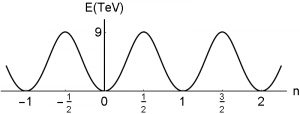
As already mentioned in my third post about the QCD vacuum, one of my favorite toy models is the quantum pendulum. It is the perfect toy model to understand the structure of the QCD vacuum and the electroweak vacuum and will be now invaluable again.

The Schrödinger equation for the quantum pendulum is

$$ – \frac{d^2 \psi}{d x^2} + g(1-cos x) \psi = E \psi . $$

We want to calculate things explicitly and therefore consider a closely related, simpler model and will come back to the full pendulum later. For small motions of the pendulum, we can approximate the potential ( $\cos(x) \approx 1-x^2/2+x^4/4! – \ldots$) of the quantum pendulum and end up with the Schrödinger equation for the anharmonic oscillator

$$ – \frac{d^2 \psi}{d x^2} – (x^2+ g x^4 )\psi = E \psi . $$

Now, the first thing we can do with this toy model is to understand Dyson’s argument from another perspective.

The potential of the anharmonic oscillator is $ V= x^2+ g x^4$ and let’s say we want to calculate the energy levels by using the usual quantum mechanical perturbation theory $E(g) = \sum_n c_n g^n $. (More precisely: The energy levels of the harmonic oscillator are well known and we are using the Rayleigh-Schrödinger perturbation theory to calculate corrections to them which come from the anharmonic term $\propto x^4$ in the potential. )

For positive values of $g$ the potential is quite boring and looks almost like for the harmonic oscillator. However, for negative values of $g$ the situation becomes much more interesting.

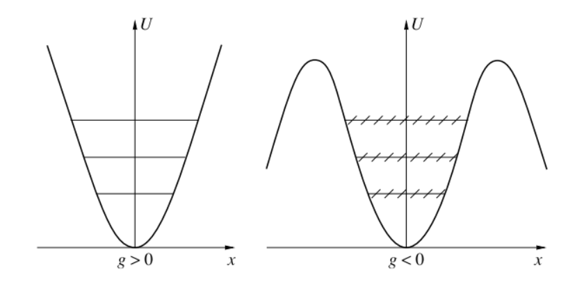
The energy is no longer bounded from below. The states inside the potential are no longer stable but can decay indefinitely by tunneling through the potential barrier. This is exactly the same situation that we discussed earlier for QED with negative $\alpha$.

Thus, according to Dyson’s argument, we suspect that the perturbation series for the energy levels is not convergent.

This was confirmed by Bender and Wu, who treated the “anharmonic oscillator to order 150 in perturbation theory“. (Phys. Rev. 184, 1231 (1969); Phys. Rev. D 7, 1620 (1973))

We can already see from the first terms in the perturbation theory how the series explodes:

$$ \rightarrow E_0 \propto \frac{1}{2} + \frac{3}{4}g – \frac{21}{8}g^2 + \frac{333}{16}g^3 + \ldots $$

This gives further support to Dyson’s conjecture that a dramatically different physics for negative values of the coupling constant means that the perturbation theory does not converge.

Yet, the story of this toy model does not end here. There is much more we can do with it.

The Anharmonic Oscillator in “QFT”

Let’s have a look how we would treat the anharmonic oscillator in quantum field theory. (This example is adapted from the excellent https://arxiv.org/abs/1201.2714). For this purpose, we consider the following “action” integral

$$\mathcal{Z}(g) = \int_{-\infty}^\infty \mathrm{d}x \mathrm{e}^{-x^2-g x^4} .$$

The cool thing is now that we can compute for this toy model the exact answer, for example, using Mathematica. Then, in a second step we can treat the same integral was we usually do in QFT and then compare the perturbative result with the exact result. Then in the last step, we can understand at what order and why the perturbation series diverges.

The full, exact solution isn’t pretty, but no problem for Mathematica:

$$ \mathcal{Z}(g) = \frac{\mathrm{e}^{\frac{1}{8g}}K_{1/4}(1/8g}{2 \sqrt{g}}, $$

where $K_n$ denotes modified Bessel function of the second kind. This solution yields a finite positive number for each value $g$.

Next, we do what we usually do in QFT. We split the “kinetic” and the “interaction” part and expand the interaction part as a power series

\begin{align}
\mathcal{Z}(g) &= \int_{-\infty}^\infty \mathrm{d}x \mathrm{e}^{-x^2-g x^4} = \int_{-\infty}^\infty \mathrm{d}x \mathrm{e}^{-x^2} \sum_{k=0}^\infty \frac{(-gx^4)^k}{k!} \notag \\
& \text{“}= \text{“} \sum_{k=0}^\infty \int_{-\infty}^\infty \mathrm{d}x \mathrm{e}^{-x^2} \frac{(-gx^4)^k}{k!} \notag
\end{align}

Take note that the exchange of sum and integral is the “root of all evil”, but necessary to interpret the theory in terms of a power series of Feynman diagrams. That’s why the last equal sign is put in quotes. (This exchange is actually a “forbidden” step that changes the behaviour at $\pm \infty$. )

So, with this approach to what extend can we get a good approximation?

Using a bit of algebra, we can solve the polyonimian times Gaussian integral and get

\begin{align}
\mathcal{Z}(g) & \text{“}= \text{“} \sum_{k=0}^\infty \int_{-\infty}^\infty \mathrm{d}x \mathrm{e}^{-x^2} \frac{(-gx^4)^k}{k!} \notag \\
&= \sum_{k=0}^\infty \sqrt{\pi} \frac{(-g)^k (4k)!}{2^{4k}(2k)! k!}
\end{align}

This perturbative answer is a series that diverges! (For more details, see the excellent detailed discussion in https://arxiv.org/abs/1201.2714)

Is this perturbative answer, although divergent, useful anyway?

Let’s have a look.

The thing is that in QFT we can only compute a finite number of Feynman diagrams. This means we can only evaluate the first few terms of the perturbation series. Thus we consider the “truncated” series, instead of the complete series, which simply means we stop at some finite order $N$:

$$ \Rightarrow \text{Truncated Series: } \mathcal{Z}_N(g) = \sum_{k=0}^N \sqrt{\pi} \frac{(-g)^k (4k)!}{2^{4k}(2k)! k!} $$

For definiteness let’s choose some value for the coupling constant, say $g=\frac{1}{50}$. How good is the perturbative answer from the truncated series compared to the full exact answer?

\begin{align}
\text{Exact: } \mathcal{Z}(1/50) &= 1.7478812\ldots \notag \\
\text{Perturbatively: } \mathcal{Z}_5(1/50) &= 1.7478728\ldots \notag \\
\mathcal{Z}_{10}(1/50) &= 1.7478818\ldots \notag
\end{align}

This is astoundingly good! The complete series is divergent, which means if we would sum up all the terms, we would get infinity. Nevertheless, if we only consider the first
few terms, we get an excellent approximation of the correct answer!

This behavior can be understood nicely by a plot

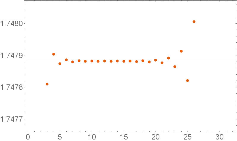
The first few terms are okay, then the approximation becomes really good, but at some point, the perturbative answer explodes. A series that behaves like this is known as an asymptotic series.

So now, the question we need to answer is:

When and why does the series diverge?

Again, I will give you a short summary of the answer first, and afterward discuss it in more detail.

The reason that the series explodes at some point is that a perturbative treatment in terms of a Taylor series misses completely factors of the form $ \mathrm{e}^{-c/g} \sim 0 + 0 g + 0 g^2 + \ldots $. The Taylor expansion of such a factor yields zero at all order, although the function obviously isn’t zero. This is a severe limitation of the usual perturbative approach.

You may wonder, why we should care about such funny looking factors. The thing is that tunneling effects in a quantum theory are described precisely by such factors! Remember, for example, the famous quantum mechanical answer of a particle that encounters a potential barrier. It will tunnel through the barrier, although classically forbidden. Inside the potential barrier, we don’t get an oscillating wave function, but instead, an exponentially damping, described by factors of the form $ \mathrm{e}^{-c/g}$.

To summarize: Our perturbative approach misses tunneling effects completely and this is why our perturbation series explodes!

We will see in a moment that this means that the divergence starts around order $N=\mathcal{O}(1/g)$. For example, in QED the perturbative approach is expected to work up to order 137.

We can understand this, by going back to our toy model. Have a look again at the quantum pendulum.

Usually, we consider small oscillations around the ground state, which means low energy states. However in a quantum theory, even at low energies, the pendulum can do something completely different. It can rotate once around its suspension. As it classically does not have the energy to do this, we have here a tunneling phenomenon. This kind of effect is what our usual perturbative approach misses completely and this is why the perturbation series explodes.

After this heuristic discussion, let’s have a more mathematical look how this comes about.

There is a third method, how we can treat our integral $\mathcal{Z}(g) = \int_{-\infty}^\infty \mathrm{d}x \ \mathrm{e}^{-x^2-g x^4}$. This third method is known as the method of steepest descend and it shows nicely what goes wrong with when we use the usual perturbative method.

First, we substitute $x^2\equiv \frac{u^2}{g}$ and then have

$$\mathcal{Z}(g) = \int_{-\infty}^\infty \mathrm{d}x \ \mathrm{e}^{-x^2-g x^4} = \frac{1}{\sqrt{g}} \int_{-\infty}^\infty \mathrm{d}u \ \mathrm{e}^{- \frac{u^2 + u^4}{g}}$$

Now, we deal with small values of the coupling $g$ and thus the integrand is large. The crucial idea behind the method of steepest descend is that the main contributions to the integral come from the extrema of the integrand $\phi(u)\equiv u^2+u^4$.

As usual, we can calculate the extrema by solving $\phi'(u_0) =0$. Take note that in QFT these extrema of our action integrand are simply the solutions to the equations of motion! (This is how we calculate the equations of motion: we look for extrema of the action. This means, $\phi'(u_0) =0$ are in QFT simply our equations of motion and the solutions $u_0$ are solutions of the equations of motion.

To approximate the integral, we then expand the integrand around these extrema. In our example, the extrema are $u=0$ an $u=\pm i/\sqrt{2}$. (For more details, see https://arxiv.org/abs/1201.2714)

This method tells us exactly what goes wrong in the usual approach. The standard perturbation theory corresponds to the expansion around $u=0$.

The other extrema yield contributions $\propto \mathrm{e}^{-\frac{1}{4g}}$ $\rightarrow$ and as already discussed earlier, these are missed completely by a Taylor series around $g=0$.

With this explicit result, we can calculate when these “non-perturbative” contributions become important.

This question in mathematical terms is: When is $\mathrm{e}^{-\frac{1}{4g}} \approx g^k $?

First, we use the log on both sides, which yields the question: When is $-\frac{1}{4g} \approx k \ \mathrm{ln}(g) $?

Now, if we have a look at some explicit numbers: $ \mathrm{ln}(1/50)\approx -3.9$, $ \mathrm{ln}(1/100)\approx -4.6$, $ \mathrm{ln}(1/150)\approx -5$, we see that the answer is: for $ k \approx \frac{1}{g}$!

Thus, as claimed earlier, the nonperturbative effects that are missed by the Taylor expansion treatment become important at order $\approx \frac{1}{g}$ and this is exactly where our perturbation series stops to make sense.

(For a nice discussion of this method of steepest descent, see page 2 here )

Before we summarize what we have found out and learned here there is one last thing.

One Last Thing

There is an amusing empirical rule related to such asymptotic series:

(Carrier’s Rule). Divergent series converge faster than convergent
series because they don’t have to converge. from The Devil’s Invention: Asymptotic, Superasymptotic and Hyperasymptotic Series by John P. Boyd

The thing is that convergence is a concept relating to the behavior at $n \to \infty$. This is not what we are really interested in. We want a good approximation by calculating just a few terms of the perturbation series, not all of them.

This kind of behavior is often observed in divergent series. They often yield good approximation at a low order, which, in contrast, is unusual for convergent power series. This is a numerical, empirical statement that was found in many explicit examples, see: Bender, C. M., and Orszag, S. A.: Advanced Mathematical Methods for Scientists and Engineers, McGraw-Hill, New York, 1978, p. 594

Thus, instead of Abel’s perspective

Divergent series are the invention of the devil, and it is shameful to base on them any demonstration whatsoever.

we should prefer Heaviside’s attitude

The series is divergent; therefore we may be able to do something with it

Summary, Conclusions, and Outlook

The thing to take away is nicely summarized by the following picture adapted from a presentation by Aleksey Cherman:

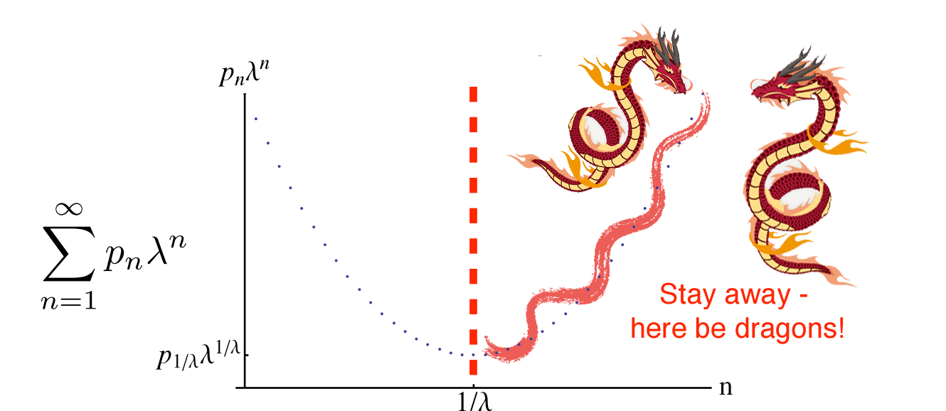
The perturbation series in QFT diverge $\sum_n^\infty c_n g^n =\infty$, but are expected to yield meaningful results up to order $N=\mathcal{O}(1/g)$.

This observation is a great reminder that perturbative Feynman diagrams don’t tell the whole story: tunneling effect, which is proportional to $\mathrm{e}^{1/g}$ are missed completely.

Dyson published his argument in 1952 so all this is known for a long time.

However, there is still a lot of research going on.

One concept people talk about all the time when it comes to this is Borel summation. This is a cool mathematical trick to improve the convergence of divergent series. For the anharmonic oscillator, this works perfectly. By performing a Borel transformation, we can tame the divergence. However, in realistic quantum field theoretical examples this does not work.

The main reason is singularities of the Borel sum. One source of these singularities are the tunneling effects we already talked about. However, much more severe are singularities coming from so-called “renormalons”. This word is used to describe the singularities coming from the renormalization procedure and thus in some sense from the running of the coupling constants.

An active field of research in this direction is “resurgence theory“. People working on this try to use a more general perturbation ansatz
$$\mathcal{O}= \sum_n c_n^{(0)} \alpha^n + \sum_i \mathrm{e}^{S_i/g} \sum_n c_n^{(i)} \alpha^n $$
called a trans-series expansion. The crucial thing is, of course, that they explicitly include the factors $\mathrm{e}^{S_i/g}$ that are missed by the usual ansatz. Thus, in some sense they try to describe “non-perturbative” effects with a new perturbation series.

At the other end of the spectrum are people working on completely non-perturbative results for observables. The most famous example is the amplituhedron, which was proposed a few years ago. This is a geometric object and the people working on it hope that it paves the way to a “nice general solution which would provide all-loop order results.” (J. Trnka)

PS: Many thanks to Marcel Köpke who spotted several typos in the original version.

Demystifying the QCD Vacuum: Part 3 – The Untold Story

Although the subtle things that are often glossed over in the standard treatment of the QCD vacuum can be explained as discussed in part 2, there is another, more intuitive way to understand it.

Most importantly, this different perspective on the QCD vacuum shines a completely new light on the mysterious $\theta$ parameter.

To the expert, this perspective will be familiar. It sometimes appears in the literature and therefore the “untold” part in the headline is, of course, a bit exaggerated. However, it took me, as a student, a long long time to find it at all and most importantly a proper explanation that made sense to me.

The standard story of the QCD vacuum uses the temporal gauge. This is not a completely fixed gauge. Time-independent gauge transformations are still allowed. Only this residual gauge freedom makes the whole discussion in terms of large and small gauge transformations, etc. possible.

One may wonder what happens when we analyze the vacuum in a different gauge, where there is no residual gauge freedom. In other words: in a gauge that fixes the gauge freedom completely. Possibly choices are, for example, the axial and the Coulomb gauge.

The interpretation of the QCD vacuum is completely different in these gauges. Most importantly: there is no vacuum periodicity.

In the axial gauge, there is only one non-degenerate ground state. Then, of course, it is natural to wonder what we can learn about the $\theta$ parameter here. At a first glance, the result that there is a unique ground state implies that we have $\theta=0$. However, this is not the case and we will discuss this in a moment.

In the Coulomb gauge, there is only a non-degenerate ground state, too. However, the interpretation of the vacuum structure in this gauge is especially tricky. Most famously, one encounters the famous Gribov ambiguities. These appear because the condition that fixes the Coulomb gauge does not lead to unique gauge potentials everywhere in spacetime. Instead, there are regions where there are multiple gauge potential configurations that satisfy the condition. These configurations are called Gribov copies and the fact that we do not get a unique gauge potential configuration everywhere in spacetime is called Gribov ambiguity.

Now, how is this not a contradiction to the standard picture of the QCD vacuum? When there is only a unique non-degenerate ground state, there is no tunneling between degenerate vacua and therefore no $\theta$ parameter, right?

No! There is still tunneling and also a $\theta$ parameter. In the axial gauge, the tunneling starts from the unique ground state and ends at the same unique ground state. (In the Coulomb gauge the tunneling happens between the Gribov copies?!)

To understand this, we need an analogy.

A nice analogy to the QCD vacuum is given by the following Hamiltonian:

$$ H= – \frac{d^2 }{d x^2} + q(1-cos x) ,$$

where $-\infty \leq x \leq \infty$ and which describes a particle in a periodic potential $V(x) = q (1-cos x)$. Therefore, this situation is quite close to the standard picture of the QCD vacuum, with a periodic structure and infinitely many degenerate ground states.

Source: https://arxiv.org/abs/1505.03690

For this Hamiltonian, we have the Schrödinger equation

$$ – \frac{d^2 \psi}{d x^2} + q(1-cos x) \psi = E \psi . $$

(Among mathematicians this equation is known as the “Mathieu equation”. Sometimes it’s useful to know the name of an equation, if you want to dig deeper.)

However, exactly the same Hamiltonian describes a “quantum pendulum”. This interpretation only requires that we treat our variable as an angular variable: $x \to \phi$, with $0 \leq \phi \leq 2 \pi$ and thus

$$ – \frac{d^2 \psi}{d \phi^2} + q(1-cos \phi) \psi = E \psi . $$

Now, we identify the point $2 \pi$ with $0$ and all values of $\phi$ that are larger than $2 \pi$, with the corresponding points in the interval $0 \leq \phi \leq 2 \pi$. This implies immediately that $ \Psi(\psi + 2\pi) = \Psi(\psi) $. Therefore, the situation now looks like this:

and we no longer have infinitely many degenerate ground states, but only a unique ground state! Therefore, the situation here is exactly the same as for the QCD vacuum in a physical gauge.

Now, what about tunneling?

For a long pendulum, i.e. for large $q$, the ground state $\psi =0$ and excited states are approximately the same as for a harmonic oscillator. For large $q$, we can do a perturbative analysis in $q^{-1/2}$ and take the “anharmonicity” this way into account. However, the famously this perturbation series does not converge, because we miss something important in our analysis. Even for a pendulum with small energy, i.e. with only small perturbations around the ground state, the pendulum can “tunnel”. In this context, this means that the pendulum does a motion that it isn’t allowed to do, like rotate once around its suspension and end up again and the ground state. This is exactly what the instantons describe in a physical gauge like the axial gauge. There is no tunneling between degenerate ground states because there are no degenerate ground states. Instead, we have tunneling that starts at the unique ground state and ends again at the unique ground state. Still, this is tunneling, because there is a potential barrier that prohibits that a pendulum rotates once completely around its suspension. For a pendulum with low energy, or equally a long pendulum (large $q$), we can do the usual quantum mechanical perturbation analysis. This yields harmonic oscillator states plus small corrections from the anharmonicity. However, we must take into account that there are also quantum processes, like the tunneling once around the suspension of the pendulum.

Okay, fine. But what about $\theta$?

Well, now that we have understood that there can also be tunneling in the physical gauge picture of the QCD vacuum, which corresponds to the pendulum interpretation of the Hamiltonian in the example above, we can argue that there can be again a $\theta$ parameter. This is the phase that the pendulum picks up when it tunnels around its suspension. In a quantum theory, we can have $\Psi(\psi + 2\pi) = e^{-i \theta} \Psi(\psi) $ instead of $ \Psi(\psi + 2\pi) = \Psi(\psi) $.

When we interpret the Hamiltonian in the example above as the movement of a particle in a periodic potential, the parameter $\theta$ describes different states in the same system, completely analogous to the Bloch momenta in solid-state physics.

However, in the pendulum interpretation different $\theta$ describe different systems, i.e. different pendulums! Thus, in this second interpretation, it is much clearer why $\theta$ is a fixed parameter and not allowed to change.

To bring this point home, let’s consider an explicit example how a $\theta$ parameter can arise for the quantum pendulum.

The pendulum only picks up a phase $\theta$, when it moves in an Aharonov-Bohm potential. To make this explicit, let’s assume the pendulum carries electric charge $e$ and rotates around a solenoid with magnetic flux $\theta$. This magnetic flux is the source of a potential $ A$ in the plane of the rotating pendulum.

We get the Hamiltonian that describes this system by replacing the derivative with the covariant derivative:

$$ H= – \left(\frac{d }{d \phi} -ie A\right)^2+ q(1-cos \phi)  ,$$

and thus we have the Schrödinger equation

$$ – \left(\frac{d }{d \phi} -ie A\right)^2 \psi+ q(1-cos \phi) \psi= E \psi .$$

As before, we impose the condition $ \Psi(\psi + 2\pi) = \Psi(\psi) $. However, we can also introduce a new wave function $\varphi (\psi) $ that obeys the standard Schrödinger equation without the additional vector potential

$$ – \frac{d^2 \varphi}{d \phi^2} + q(1-cos \phi) \varphi = E \varphi ,$$

where

$$ \psi(\phi) = \text{exp} \left[ ie \int_0^\phi A d\phi \right] \varphi(\phi).$$

(Take note that the relation between the magnetic flux $\theta$ and the potential $A$ is $ \int_0^{2\pi} A d\phi = \theta $).

The information about the presence of the magnetic flux and hence of the vector potential $ A$ is now, when we use $\varphi(\phi)$ instead of $\Psi (\phi)$, encoded in the boundary condition:

$$ \varphi(\phi + 2\pi) = e^{-ie\theta} \varphi(\phi). $$

The energy of the ground state of the pendulum is directly proportional to the magnetic flux:

$$ E (\theta) \propto (1- \cos(\theta)) .$$

This show that in this model, the parameter $\theta$ defines different systems, namely quantum pendulums in the presence of different Aharonov-Bohm potentials.

In contrast, in the periodic potential picture, where $\theta$ is interpreted as analogon to the Bloch momentum, the parameter $\theta$ describes different states of the same system.

The reinterpretation of the QCD vacuum in a physical gauge with a unique non-degenerate vacuum, thus makes the appearance of $\theta$ much less obvious. This is why the standard presentation of the topic still makes use of the temporal gauge and the periodic vacuum picture.

The analysis of the QCD vacuum in the axial gauge is analogous to the interpretation of the Hamiltonian $$ H= – \frac{d^2 }{d \phi^2} + q(1-cos \phi) $$ as description of a quantum pendulum, i.e. substituting $x \to \phi$, with $0\leq \phi < 2 \pi$. (This interpretation also arises, when we work in the temporal gauge and declare that all gauge transformations (large and small) should not have any effect on the physics. The distinct degenerate vacua in the usual interpretation are connected by large gauge transformations. )

Without any further thought, one reaches immediately the conclusion that there is no $\theta$ parameter here. However, this is not correct, because a $\theta$ parameter can appear when there is an Aharonov-Bohm potential present.

When the quantum pendulum swings in such a potential, it picks up a phase when it rotates once around the thin solenoid that encloses the magnetic flux. The phase is directly proportional to the magnetic flux in the solenoid.

For the QCD vacuum, the same story goes as follows. In the axial gauge, naively there is no $\theta$ parameter because we do not have a periodic potential and hence no Bloch-momentum. However, nothing forbids that we add the term

$$ – \frac{g^2 \theta}{32\pi^2} Tr(G_{\mu\nu} \tilde{G}^{\mu\nu}),$$

where $\tilde{G}^{\mu\nu}$ is the dual field-strength-tensor: $\tilde{G}^{a,\mu \nu} = \frac{1}{2} \epsilon^{\mu \nu \rho \sigma} G^a_{ \rho \sigma}$, to the Lagrangian. This simply means that we allow for the possibility that there is an Aharonov-Bohm type potential and that it could make a difference when the pendulum rotates once around its suspension.

An obvious question is now, what the analogon to the solenoid is for the QCD vacuum. So far, I wasn’t able to find a satisfactory answer. The usual argument for the addition of $ – \frac{g^2 \theta}{32\pi^2} Tr(G_{\mu\nu} \tilde{G}^{\mu\nu})$ to the Lagrangian is that nothing forbids its existence.

So far, all experimental evidence point in the direction that there exists no “solenoid” for the QCD vacuum and therefore $\theta =0$. (The current experimental bound is $\theta < 10^{-10}$, Source).

From the analysis of the QCD vacuum in the axial gauge and by comparing it to the quantum pendulum, this does not look too surprising. However, we shouldn’t be too quick here and state $\theta =0$. Before we can say something like this, we need to understand first, what the “solenoid” could be for the QCD vacuum.

Understanding this requires that we enter a completely different world: the world of anomalies. This fascinating topic deserves its own post. Usually, it is claimed that the contribution to $\theta$ that comes from this sector of the theory is completely unrelated to the QCD $\theta$. However, we will see that anomalies and the QCD vacuum aren’t that unrelated: So far, we were only concerned with the gauge boson vacuum, while anomalies arise when we consider the fermion vacuum and its interaction with gauge bosons!

This will be discussed in part 4 of my series about the QCD vacuum.

References that describe this perspective of the QCD vacuum

  • “Topology in the Weinberg-Salam theory” by N. S. Manton
  • “The Interpretation of Pseudoparticles in Physical Gauges” by Claude W. Bernard, Erick J. Weinberg
  • Section 11.3 in Rubakov’s “Classical Theory of Gauge Field”
  • This perspective of the QCD vacuum in more abstract terms without the quantum pendulum analogy is described in “Introduction to the Yang-Mills Quantum Theory” by R. Jackiw in the around Eq. (42).

Demystifying the QCD Vacuum: Part 2 – The Subtleties No One Talks About

This is part two of my series about the QCD vacuum. You should only read this if you are confused about several things that are glossed over in the standard treatments. It turns out, that if you dig a bit deeper, these several such small things aren’t as obvious as most authors want you to believe. I already mentioned the problems with the two assumptions that are made in the standard texts without proper explanations. Here I will discuss the assumptions in more detail.

My main focus is answering the questions: Why there is so much emphasize on gauge transformations that become trivial at infinity $g(r, \phi , \theta) \to 1 $ for $r \to 1$ and why do the usual discussions make use of the temporal gauge? I already discussed in the first post, why these assumptions are absolutely crucial. Without them, there is no way to arrive at the standard interpretation of the QCD vacuum.

These two things only make sense, when you know something about constrained Hamiltonian quantization and Gauss’ law.

Only if you have some basic understanding of these two notions, you can truly understand the ideas of the discoverers of the non-trivial structure of the QCD vacuum.

My plan is to write more about both, constrained Hamiltonian quantization and Gauss’ law, in the future, but just to demonstrate that both are an interesting topic on their own, regardless of the QCD vacuum, here are two quotes:

“The constrained Hamiltonian formalism is recommended as a means for getting a grip on the concepts of gauge and gauge transformation. This formalism makes it clear how the gauge concept is relevant to understanding Newtonian and classical relativistic theories as well as the theories of elementary particle physics; it provides an explication of the vague notions of “local” and “global” gauge transformations; it explains how and why a fibre bundle structure emerges for theories which do not wear their bundle structure on their sleeves; it illuminates the connections of the gauge concept to issues of determinism and what counts as a genuine “observable”; and it calls attention to problems which arise in attempting to quantize gauge theories. “ Gauge Matters by John Earman


“The main output of this analysis is therefore the suggestion that Gauss law is the basic and primary feature which characterized elementary particle interactions, rather than gauge invariance, a concept which is more difficult to grasp on physical grounds since it can be given a meaning only by introducing unobservable quantities. Gauge Invariance can therefore be regarded as a technical tool for constructing Lagrangian functions or equations of motion which guarantee the validity of Gauss’ law. This may be the right track to get an insight into the structure of GQFT and possibly understand why nature seems to choose gauge theories for elementary particle interactions.”
Gauss’ Law in Local Quantum Field Theory by F. Strocchi

This post should be about how these concepts help to understand the standard discussion of the QCD vacuum and therefore I will keep discussions that would lead us too far apart to a minimum.

So, without further ado, let’s get started.

How do we get a Quantum Theory?

In modern physics, when we write down a model to describe a given system, we start with a Lagrangian. This is clever because the Lagrangian framework is ideal to make use of symmetry considerations. If the Lagrangian (or better, the action) is invariant under some transformation, the equations of motion, have this symmetry, too.

In contrast, for example, the Hamiltonian, is not even invariant under Lorentz transformations as it represents the energy and is thus only one component of a Lorentz vector, the four momentum. Therefore, it is much harder to “guess” the correct Hamiltonian that describes the system in question.

However, when we want to describe a quantum system, a Lagrangian is not enough. Although we get from the Lagrangian the equations of motion via the Euler-Lagrange equations, these are not enough to describe the quantum behavior of the system. The equations of motions are, on their own, purely classical and there is nothing quantum about them.

Thus, we need additional equations that describe the quantum behavior and we get them through the process called “quantization”.

There are different ways to quantize a given classical system, but one popular and famous possibility is the constrained Hamiltonian quantization procedure. (A now-popular alternative is the path-integral formalism. However, the canonical procedure described below makes many points more transparent).

This is a reliable way to quantum physics and the main points are well known to most students. We derive from the Lagrangian the canonical momenta and then quantize the system by replacing the classical Poisson bracket with the quantum commutator (or anticommutator)

$$ \{ \cdot , \cdot \} \to \frac{1}{i\hbar} [\cdot , \cdot ]. $$

However, there are several subtle points that need to be taken care of when we try to use this procedure.

While you may not care about such “details”, it is absolutely crucial to understand this procedure, if you want to understand the standard picture of the QCD vacuum that is repeated in almost all textbooks and reviews. In addition, hopefully, the quote above has sparked some interest that there is something deep that we can learn here.

For our purpose here, however, it is only important to know that the guys who came up with the standard interpretation of the QCD vacuum cared about this procedure a lot.

To (canonically) quantize, we must compute the generalized momenta $p_i$ for the given Lagrangian and then impose the famous commutation relations $[q_i,p_j]= i \delta_{ij}$.

We also need these generalized momenta to get the Hamiltonian that corresponds to the given Lagrangian. We need the Hamiltonian in the canonical formalism, for example, to calculate the time-evolution of quantum fields.

The mathematical procedure to get the Hamiltonian from a given Lagrangian and thus to get the generalized momenta is called Legendre transform.

However, this procedure is not as straight-forward as one would naively assume. The Lagrangian is a function of $q_i$ and $\dot{q}_i$, whereas the Hamiltonian is a function of $q_i$ and the generalized momenta and $p_i$. The Legendre transform is the process to calculate from the generalized velocities $\dot{q}_i$ the corresponding generalized momenta $p_i$:

$$ p_i \equiv \frac{\partial L }{\partial \dot{q}_i} .$$

In principle, we can invert this definition and get the generalized velocities as a function of $q$ and $p$: $ \dot{q}_i = \dot{q}_i (q_i,p_i)$.

However, for some systems, these relations are not invertible. Instead, not all momenta are independent and we get a family of constraints that the momenta must satisfy

$$ f_a(q,p) =0 \quad a=1,…,N $$

These constraints are the reason why this formalism is called constrained Hamiltonian quantization.

Glossing over some details (the process of finding all independent constraints and the definition of “first-class” constraints, which are those constraints whose mutual Poisson bracket vanishes), the crucial thing is now that the constraints generate gauge transformations!

The understand this, we note that the correct total Hamiltonian is given by the “naive” Hamiltonian $H_T$ plus a linear combination of all (first class) constraints with arbitrary coefficients

$$ H_T = p_i \dot{q}_i – L + \sum_{a=1}^N \lambda_a(t) f_a.$$

(The implementation of constraints in this way is known as the method of “Lagrange multiplies”)

The Hamiltonian describes the time evolution of the system in question. The additional terms here mean that there is an ambiguity in the time evolution and this ambiguity is exactly our gauge freedom!

The origin of these complications, can be traced back to the equations of motions in the Lagrangian framework

$$ \frac{\partial^2 L}{\partial \dot{q}_i \partial \dot{q}_j } \ddot{q}_j= – \frac{\partial^2 L}{\partial \dot{q}_i \partial q_j } \dot{q}_j + \frac{partial L}{\partial q} . $$

The accelerations can only be determined in terms of the positions and velocities if the Jacobian matrix of the transformation $(q_i, \dot{q}_i) \to (p_i, p_i)$:

$$\frac{\partial p^i}{\partial \dot{q}_j} = \frac{\partial^2 L}{\partial \dot{q}_i \partial \dot{q}_j } \ddot{q}_j$$

is non-singular. Only then, the transformation is unique and the canonical quantization procedure works without subtleties.

This can be seen, by analyzing the equation $\det\left( \frac{\partial^2 L}{\partial \dot{q}_i \partial \dot{q}_j } \ddot{q}_j \right) =0 $. This equation implies that some of the momenta aren’t independent variables.

This means, we have constraints when the determinant of the Jacobian matrix is zero and therefore the time evolution is not uniquely determined in terms of the initial conditions.
(For more on this, see, for example, this paper).

This is a very special perspective on gauge freedom that isn’t very familiar to students nowadays. However, it is absolutely crucial to understand what the discoverers of the non-trivial structure of the QCD vacuum had in mind.

A concrete example may be helpful.

Constrained Quantization of Electrodynamics

The Lagrangian of electrodynamics is $L = – \frac{1}{4} \int d^3xF_{mu\nu} F^{\mu\nu}$ and contains some gauge freedom. This becomes especially transparent when we try to quantize electrodynamics by following the procedure described above.

The path from this Lagrangian to the correct description in the Hamiltonian framework is quite subtle because we have here an explicit example, of the situation described above.

When we calculate the generalized momenta to $A_\mu$:

$$ \pi^\mu = \frac{\partial L}{\partial (\partial_0 A_\mu)}= F^{\mu 0}, $$

we get $\pi^0 =0$ and $\pi = E^i$, where $E$ is the usual electric field. Thus, we notice here the constraint: $\pi^0 =0$.

Following, the procedure described above, we have the following total Hamiltonian
$$ H_T = \int d^3x \left( \pi^\mu \partial_0 A_\mu – \mathcal{L} \right) + \int d^3x \lambda_1(x) \pi_0(x)$$
$$ \int d^3 x \left( \frac{1}{2} (\vec{E}^2 +\vec{B}^2) + A_0 \Delta \cdot \vec E \right) + \int d^3x \lambda_1(x) \pi_0(x) $$

(In this calculation, one uses $\partial_0 \vec A = \Delta A_0 -\pi = \Delta A_0 – \vec E$ and integrates the second term by parts.)

We recognize the first term here $\propto \frac{1}{2} (\vec{E}^2 +\vec{B}^2)$ as the well known electromagnetic field energy density. The last term is the implementation of the constraint $\pi_0(x) =0$ via a Lagrange multiplier $\lambda_1(x)$. What about the second term?

To understand this second term, let’s take a step back and go back to the Lagrangian.

One of the equations of motions that we get via the Euler-Lagrange equations from the Lagrangian $L = – \frac{1}{4} \int d^3xF_{mu\nu} F^{\mu\nu}$, is Gauss’ law:

$$ \Delta \cdot \vec E = 0. $$

(Gauss’ law is, of course, one of the famous Maxwell equations. In words, Gauss law simply states that the flux of the electric field from a volume is proportional to the charge inside. In electrodynamics without sources, which is what we consider here with our Lagrangian, this flux is therefore zero.)

However, take note that it is a very special kind of “equation of motion”. It contains no time-derivatives and therefore does not describe any time-evolution. Hence it is not really an equation of motion!

If we now have again a look at the Hamiltonian that we derived above, we can see that the second term has exactly the same structure as the third term. The equation $ \Delta \cdot \vec E = 0$ is a constraint, exactly as $\pi_0(x) $. The Lagrange multiplier for this term is simply $A_0(x)$.

Our two (first class) constraints are $\pi_0 =0$ and $\Delta \vec{\pi } = \Delta \vec{E}=0$. In the Hamiltonian framework, they show up as constraints that we implement by making use of Lagrange multipliers.

Now that we know that $A_0(x)$ is not really a dynamical variable, it seems reasonable to simplify our calculations by choosing the temporal gauge $A_0(x)=0$. (It can already be seen from the Lagrangian that $A_0(x)$ is not a dynamical variable because there is no time derivative of $A_0(x)$ in the Lagrangian.)

However, $A_0(x)=0$ is not a complete gauge fixing. We still have the freedom to perform time-independent gauge transformations. This remaining gauge freedom can be fixed, for example, by the demand $\Delta \cdot \vec A =0$.

When we recall the remark from above, that the constraints generate gauge transformations, we can understand the residual gauge freedom after fixing $A_0(x)=0$ from another perspective:

The choice $A_0(x)=0$ uses up the gauge freedom generated by $\pi_0 =0$ (called the momentum constraint). However, we still have the gauge freedom generated by Gauss’ law $\Delta \vec{E}=0$.

This can be seen, for example, by going back to the Lagrangian invoking Noether’s theorem for time-independent gauge transformations.

The conserved “charge” that follows from invariance under time-independent gauge transformations:

$$ Q_\phi = \int dr \pi_a \cdot \delta A_a = \frac{1}{g} \int_{-\infty}^\infty dr \vec {E}_a (\Delta \phi (r))_a $$

where $\phi(x)$ is the “gauge function”. This looks almost like Gauss’ law, but not exactly. Gauss law involves $\Delta \vec{E}$, whereas here $\Delta $ acts on the gauge function $\phi(x)$. However, we can rewrite this Noether charge such that it contains $\Delta \vec{E}$ by integrating by parts.

When we integrate by parts, we get a boundary term $( \frac{1}{g} \vec {E}_a \phi (r)_a \big |_{-\infty}^\infty $. We can only neglect this boundary term, when $\phi (-\infty) = \phi (\infty) =0$.

This is a subtle point that is often glossed over (see, for example, Eq. 3.22 in Topological investigations of quantized gauge theories by R. Jackiw, where this “glossing over” is especially transparent). The subtle and small observation that $\theta (-\infty) = \theta (\infty) =0$ is a requirement for Gauss’ law to be a generator of gauge transformations will become incredibly important in a moment.

Forgetting this “detail” for a moment, we can conclude $ E_a\cdot \Delta$ is conserved. This can also be verified, by computing the explicit commutator with the Hamiltonian. Noether charges always generate the corresponding symmetry transformations and in this sense, $ E_a\cdot \Delta$ generates time-independent gauge transformations. The Noether “charge” for time-independent gauge transformations is $\propto \Delta E$ and hence this is the generator of such gauge transformations.

(A second possibility to see that Gauss’ law generates gauge transformations is to consider the explicit commutator of $G_a = – \frac{1}{g} (\Delta E)$ and the electrical potential $A_b$ and the electrical field $E_a$. Moreover, we can compute that $\frac{i}{\hbar} [H,G_a]=0$ and therefore $G_a$ is indeed conserved. )

Gauss’ Law in a Quantum Theory

Now, let’s remember that we want to talk about a quantum theory. It is somewhat a problem what to make of Gauss’ law in a quantum theory.

On the one hand, we can invoke the equal-time commutation relations and compute

$$ [G_a (x_1),A_1(x_2)]_{t=0} = i \partial_{x_1} \delta (x_1-x_2) \neq 0 .$$

On the other hand, we have the explicit statement of Gauss’ law, that $ G_a = \Delta \cdot \vec E_a = 0$

The crucial idea to resolve this “paradox” is to take the idea that Gauss’ law is a constraint seriously. Hence, the operator $G_a$ is not zero, but when it acts on states we get zero.

In the classical theory, Gauss’ law is a restriction on the initial data. In the quantum theory, we now say that Gauss’ law defines physical states, via the equation $G |\Psi\rangle_{phys}=0$. Non-physical states can, by definition, do whatever they want and there is no need that they respect Gauss’ law. (This is the crucial idea behind the Gupta-Bleuler formalism).

Okay, this was a long convoluted story. What’s the message to take away here?

The Crucial Points to Take Away

The crucial point is that Gauss’ law only forces gauge equivalence under gauge transformations which are generated by $G_a$ and become trivial at spatial infinity.

Certainly, there are other possibly gauge transformations, but Gauss’ law has nothing to say about them.

Quantization is a science on its own and this post is not about quantization. However, I hope the few paragraphs above, make clear that when you come from the constrained Hamiltonian quantization perspective a few things are quite natural:

– $A_0(x) =0$ is an obvious choice to simplify further calculations.
– The residual gauge freedom after fixing $A_0(x) =0$ is generated by Gauss’ law. This gauge freedom includes only a very particular subset of gauge transformations. In the discussion above, we have seen that Gauss’ law only generates gauge transformations via $\text{exp}\left(\frac{1}{g} \int d^3 x \phi(\vec x)_a G_a\right)$ that include a gauge function that vanishes at infinity $\phi (-\infty) = \phi (\infty) =0$. When you come from the perspective of constrained Hamiltonian quantization, it makes sense to treat those gauge transformations that involve a gauge function that does become zero at spatial infinity as special. All other gauge transformations are not forced by Gauss law to leave physical states invariant.

Why Only Trivial Gauge Transformations?

Take note that we still haven’t fully elucidated that assumptions that were used in the first post to explain the standard story of the QCD vacuum.

So far, we have only seen why the gauge transformations with a gauge function that satisfies $\phi (-\infty) = \phi (\infty) =0$ is special because it is forced by Gauss’ law to be a symmetry of physical states.

We still have to talk about, why we restricted ourselves in the first post those gauge transformations that involve a gauge function that becomes a multiple of $2 \pi$ at spatial infinity, instead of all gauge transformations.

In other words, why was it sufficient to restrict ourselves to gauge transformations that become trivial at infinity $g(x) \to 1 $ for $|x| \to \infty$?

If you look through the literature, you will find many reasons. However, if you find many arguments, this is usually a red flag that things aren’t as bulletproof as people would like them to be.

I’m not the only one who feels this way. For example, Itzykson and Zuber write in their famous QFT book:

“there is actually no very convincing argument to justify this restriction”.

In addition, while Roman Jackiw (one of the founding fathers of the standard picture of the QCD vacuum) claimed in the original paper that this restriction $g(x) \to 1 $ for $|x| \to \infty$ simply follows because “we study effects which are local in space” (1976), he later became more careful. In his “Introduction to Yang-Mills theory” (1980) he wrote

We shall make a very important hypothesis concerning the physically admissible finite transformations. While some plausible arguments can be given in support of this hypothesis (see below) in the end we must recognize it as an assumption, without which the subsequent development cannot be made. We shall assume that the allowed gauge transformation matrices U tend to a definite limit as r passes to infinity

$$ lim_{r\to\infty} U(r)= U_\infty$$

Here $ U_\infty$ is a global (position-independent) gauge transformation matrix. With this hypothesis, we are excluding gauge transformations which do not have a well-defined or unique limit at $r \to \infty$.”

He then lists three arguments why this restriction is plausible. This is good style, but unfortunately, most other presentations of the QCD vacuum gloss over this important point and act like the restriction is obvious for some reason.

In fact, I have collected an even longer list with around 10 arguments that are put forward in textbooks and papers to justify the restriction $g(x) \to 1 $ for $|x| \to \infty$. Some are better than others and I think one is really strong, but ultimately one needs to admit that this restriction

“has always been recognized as weak but it had seemed necessary.” (Source)

Unfortunately, this recognition has not been loud and clear enough. Many students I have talked to think that this restriction has something do with the fact that we investigate “finite energy” solutions of the Yang-Mills equations. This, however, can not be correct, because the energy shouldn’t care about gauge transformations at all. Hence, there can be no reason that follows from some energy argument for the restriction to a subset of gauge transformations.

Another popular argument is that we need some boundary conditions and that our particular choice shouldn’t matter because we do not care about what happens at infinity. (See for example page 166 in “Quarks, leptons and gauge fields” by Huang, where he writes “It is a common article of faith to assume that boundary conditions at large distance have no effect on local phenomena”.). This argument is exactly what Jackiw proposed in his first paper I quoted above. However, this argument is hardly satisfactory. Our choice of boundary conditions shouldn’t make any difference. However, when we do not restrict ourselves to the subset that satisfies $g(x) \to 1 $ for $|x| \to \infty$, there is no homotopy discussion possible and the usual periodic vacuum picture does not emerge. Hence the boundary condition seems to make a big difference. Another way to see that this argument is problematic is to consider different definite boundary conditions. If they do not matter, so why not? For example, instead of $g(x) \to 1 $ for $|x| \to \infty$, which leads to a compactification of space to the sphere $\mathbb{R}^3 \to S^3$, we could consider a large box and impose periodic boundary conditions. Then space does not become a sphere, but a torus and the homotopy classification is completely different.

My favorite point of view is to ignore all these nasty things, by analyzing the QCD vacuum from a completely different perspective. I will describe this alternative description in the next post in this series.

But for now, how can we make sense of the restriction $g(x) \to 1 $ for $|x| \to \infty$?

We already know that the gauge transformations that involves a gauge function that becomes zero at infinity are special, because these are generated by Gauss’ law and hence are true symmetries of the physical states.

With this in mind, probably the best argument is that tunneling does only happens from a vacuum with winding number zero (i.e. one that is “Gauss’ law gauge equivalent” to $A_\mu =0$), to a vacuum state with integer winding number (i.e. one that we get from $A_\mu =0$ with a gauge transformation that satisfies $g(x) \to 1 $ for $|x| \to \infty$). If we can show this, it seems reasonable that we neglect other ground states are not reachable by tunneling processes.

To show this, imagine spacetime as a cylinder. Each slice of the cylinder is the complete space $\mathbb{R}^3$ at a given time $t$. The lower cap of the cylinder is space at $t = – \infty$ and the upper cap space at $t = \infty$. Now, we start at $t= -\infty$ with our quantum field in a vacuum configuration with winding number zero. We have the gauge freedom to choose $A_\mu (\vec x , -\infty) =0$. (However, take note that all other pure gauge configurations, that are generated by a Gauss’ law gauge transformation are equally valid. The gauge transformations generated by Gauss’ law are those that have a gauge function in the exponent that satisfies $f(x) \to 0$ for $|x| \to \infty$. All configurations that we get from $A_\mu(\vec x , -\infty) =0$ with such a gauge transformations are also winding number zero configurations, because they are gauge equivalent to $A_\mu(\vec x , -\infty) =0$.) Each pure gauge configuration of $A_\mu$, which means $A_\mu = U^\dagger (\vec x, t)\partial U(\vec x, t) $, is a vacuum configuration. $A_\mu (\vec x , -\infty) =0$ means $U(\vec x, -\infty) =\text{const}. $

This is the naive vacuum configuration and we want to investigate what non-trivial configurations of our quantum field are possible. We are especially interested in what the final configurations at $t = \infty$ can be.

Now, remember that we work in the temporal gauge. As already mentioned above, this choice of gauge does not fix the gauge freedom completely, but instead all time-independent gauge transformations are still permitted.

In addition, we are interested in finite energy processes. This requirement means that at spatial infinity our field energy must vanish, which means that our quantum field must be in a pure gauge configuration at spatial infinity. (This is discussed in more detail in the first post).

We now put these three puzzle pieces together:

At $t = – \infty$, we have $A_\mu(\vec x , -\infty) =0$ and therefore $U(\vec x, -\infty) =\text{const}. $ At the boundary, $A_\mu$ must stay pure gauge all the way from $t= – \infty$ to $t=\infty$: $A_\mu(\infty, t) = U^\dagger (\infty, t)\partial U(\infty, t) $.

The crucial thing is now that at $t = -\infty$, we started with a configuration that corresponds to $U(\vec x, -\infty) =\text{const}$. Thus at this time, we also have at spatial infinity $U(\infty, -\infty) =\text{const}$. In the temporal gauge, only time-independent gauge transformations are permitted. Therefore, $U(\infty, -\infty) =\text{const} = U(\infty, t) = U(\infty)$ is fixed and does not change as we time moves on!

Therefore, we also have at the upper cap of the cylinder, i.e. at $t=\infty$ are pure gauge configuration (because we consider a vacuum state to vacuum state transition) $A_\mu(\infty, \infty) = U^\dagger (\infty, \infty)\partial U(\infty, \infty) $ with $U(\infty, -\infty) =\text{const}$.

Hence, when we start with a vacuum configuration, which means a gauge transformation of $A_\mu =0$ with $U(\vec x, -\infty) =\text{const}$, our field can only transform into configurations that are gauge transformations of $A_\mu =0$ with $U(\vec x, \infty) =\text{const}$.

You may now wonder why the anything non-trivial is possible at all. The answer is that the restriction that $A_\mu$ must be pure gauge only holds:

– At the lower cap, i.e. for $A_\mu(\vec x , -\infty)$, because we start with a vacuum configuration.
– At the curved surface boundary of the cylinder, i.e. for $A_\mu(\infty, t)$, because we only consider finite energy process, which requires that the field energy vanishes at spatial infinity and thus that $A_\mu$ is pure gauge there.
– At the upper cap $A_\mu(\vec x , \infty)$, because we investigate vacuum to vacuum transitions.

Thus, in between, there is a lot of non-trivial stuff that can happen. Especially, on the way from the pure gauge at $t=-\infty$ to pure gauge $\infty$ it can be in non-pure-gauge configurations somewhere in space at some point in time. In other words, it is possible, within our restrictions that the field is, on the way from $t=-\infty$ to $t=\infty$, in a configuration that corresponds to non-zero field energy. These non-zero field energy configurations are exactly the potential barrier that we talked about in the first post. In this sense, we are dealing here with tunneling phenomena. We start with a vacuum state, i.e. zero field energy. Nevertheless, the field manages to get into configurations that “normally” would require energy to get into. However, because we are dealing with a quantum theory, it is possible that the field tunnels through these, classically forbidden configurations.

Only because this is, in principle possible, does not mean that it actually happens. However, there are solutions of the Yang-Mills equations that exactly describe such processes: the famous instanton solutions. Thus it seems reasonable that such tunneling indeed happens. (It is really cool to see how an instanton solution describes the process of how a vacuum configuration transforms into a different vacuum configuration. Different here means with a different winding number. However, there are already good descriptions in the literature and I’m currently not motivated to write down all the required formulas. An especially nice and explicit description can be found on page 168 (section 8.6.2 “Instantons as Tunneling Solutions”) in “Quarks, Leptons & Gauge Fields by Kerson Huang).

The crucial message of the description above is that we necessarily get a final field configuration that corresponds to a pure gauge configuration with $U(\vec x, \infty) =\text{const}$. The constant is necessarily the same constant that we started with at $t=-\infty$. Therefore, transitions only happen between pure gauge configurations that are generated by gauge transformations which have the same trivial limit at spatial infinity. (Trivial means that there is no dependence on angles, but instead the gauge transformation becomes the same constant no matter from which direction we approach $|x| = \infty$. )

Now, let’s connect this discussion with our previous discussion of Gauss’ law:

Recall that above we argued that the gauge transformations generated by Gauss’ law are somewhat special because we use Gauss’ law to identify physical states in a quantum theory. These gauge transformations are exactly those with a gauge function $f(x)$ in the exponent that becomes zero at spatial infinity: $U(x) = e^{if(x) \hat r \cdot \vec G}$ with $f(\infty) =0$. The naive vacuum configuration is $A_\mu=0$. All configurations that we get by transforming this configuration with a gauge transformation that is generated by Gauss’ law are completely equivalent to $A_\mu =0$, because that’s how we use Gauss’ law in a quantum theory. Therefore, starting from the naive vacuum configuration, or one that is physically equivalent, we have $U(\infty , – \infty) = 1$. Therefore, with the arguments from above, we can only end up in a configuration with $U(\infty, \infty)=1$, too!

In this sense, it is sufficient to restrict ourselves to gauge transformations that satisfy $U(x) \to 1$ for $|x| \to \infty$. This is the moral of this long story.

In my next post about the QCD vacuum, I will present another way to look at it. With this different interpretation, we can avoid all the confusing details