This is part two of my series about the QCD vacuum. You should only read this if you are confused about several things that are glossed over in the standard treatments. It turns out, that if you dig a bit deeper, these several such small things aren’t as obvious as most authors want you to believe. I already mentioned the problems with the two assumptions that are made in the standard texts without proper explanations. Here I will discuss the assumptions in more detail.
My main focus is answering the questions: Why there is so much emphasize on gauge transformations that become trivial at infinity $g(r, \phi , \theta) \to 1 $ for $r \to 1$ and why do the usual discussions make use of the temporal gauge? I already discussed in the first post, why these assumptions are absolutely crucial. Without them, there is no way to arrive at the standard interpretation of the QCD vacuum.
These two things only make sense, when you know something about constrained Hamiltonian quantization and Gauss’ law.
Only if you have some basic understanding of these two notions, you can truly understand the ideas of the discoverers of the non-trivial structure of the QCD vacuum.
My plan is to write more about both, constrained Hamiltonian quantization and Gauss’ law, in the future, but just to demonstrate that both are an interesting topic on their own, regardless of the QCD vacuum, here are two quotes:
“The constrained Hamiltonian formalism is recommended as a means for getting a grip on the concepts of gauge and gauge transformation. This formalism makes it clear how the gauge concept is relevant to understanding Newtonian and classical relativistic theories as well as the theories of elementary particle physics; it provides an explication of the vague notions of “local” and “global” gauge transformations; it explains how and why a fibre bundle structure emerges for theories which do not wear their bundle structure on their sleeves; it illuminates the connections of the gauge concept to issues of determinism and what counts as a genuine “observable”; and it calls attention to problems which arise in attempting to quantize gauge theories. “ Gauge Matters by John Earman
“The main output of this analysis is therefore the suggestion that Gauss law is the basic and primary feature which characterized elementary particle interactions, rather than gauge invariance, a concept which is more difficult to grasp on physical grounds since it can be given a meaning only by introducing unobservable quantities. Gauge Invariance can therefore be regarded as a technical tool for constructing Lagrangian functions or equations of motion which guarantee the validity of Gauss’ law. This may be the right track to get an insight into the structure of GQFT and possibly understand why nature seems to choose gauge theories for elementary particle interactions.” Gauss’ Law in Local Quantum Field Theory by F. Strocchi
This post should be about how these concepts help to understand the standard discussion of the QCD vacuum and therefore I will keep discussions that would lead us too far apart to a minimum.
So, without further ado, let’s get started.
How do we get a Quantum Theory?
In modern physics, when we write down a model to describe a given system, we start with a Lagrangian. This is clever because the Lagrangian framework is ideal to make use of symmetry considerations. If the Lagrangian (or better, the action) is invariant under some transformation, the equations of motion, have this symmetry, too.
In contrast, for example, the Hamiltonian, is not even invariant under Lorentz transformations as it represents the energy and is thus only one component of a Lorentz vector, the four momentum. Therefore, it is much harder to “guess” the correct Hamiltonian that describes the system in question.
However, when we want to describe a quantum system, a Lagrangian is not enough. Although we get from the Lagrangian the equations of motion via the Euler-Lagrange equations, these are not enough to describe the quantum behavior of the system. The equations of motions are, on their own, purely classical and there is nothing quantum about them.
Thus, we need additional equations that describe the quantum behavior and we get them through the process called “quantization”.
There are different ways to quantize a given classical system, but one popular and famous possibility is the constrained Hamiltonian quantization procedure. (A now-popular alternative is the path-integral formalism. However, the canonical procedure described below makes many points more transparent).
This is a reliable way to quantum physics and the main points are well known to most students. We derive from the Lagrangian the canonical momenta and then quantize the system by replacing the classical Poisson bracket with the quantum commutator (or anticommutator)
$$ \{ \cdot , \cdot \} \to \frac{1}{i\hbar} [\cdot , \cdot ]. $$
However, there are several subtle points that need to be taken care of when we try to use this procedure.
While you may not care about such “details”, it is absolutely crucial to understand this procedure, if you want to understand the standard picture of the QCD vacuum that is repeated in almost all textbooks and reviews. In addition, hopefully, the quote above has sparked some interest that there is something deep that we can learn here.
For our purpose here, however, it is only important to know that the guys who came up with the standard interpretation of the QCD vacuum cared about this procedure a lot.
To (canonically) quantize, we must compute the generalized momenta $p_i$ for the given Lagrangian and then impose the famous commutation relations $[q_i,p_j]= i \delta_{ij}$.
We also need these generalized momenta to get the Hamiltonian that corresponds to the given Lagrangian. We need the Hamiltonian in the canonical formalism, for example, to calculate the time-evolution of quantum fields.
The mathematical procedure to get the Hamiltonian from a given Lagrangian and thus to get the generalized momenta is called Legendre transform.
However, this procedure is not as straight-forward as one would naively assume. The Lagrangian is a function of $q_i$ and $\dot{q}_i$, whereas the Hamiltonian is a function of $q_i$ and the generalized momenta and $p_i$. The Legendre transform is the process to calculate from the generalized velocities $\dot{q}_i$ the corresponding generalized momenta $p_i$:
$$ p_i \equiv \frac{\partial L }{\partial \dot{q}_i} .$$
In principle, we can invert this definition and get the generalized velocities as a function of $q$ and $p$: $ \dot{q}_i = \dot{q}_i (q_i,p_i)$.
However, for some systems, these relations are not invertible. Instead, not all momenta are independent and we get a family of constraints that the momenta must satisfy
$$ f_a(q,p) =0 \quad a=1,…,N $$
These constraints are the reason why this formalism is called constrained Hamiltonian quantization.
Glossing over some details (the process of finding all independent constraints and the definition of “first-class” constraints, which are those constraints whose mutual Poisson bracket vanishes), the crucial thing is now that the constraints generate gauge transformations!
The understand this, we note that the correct total Hamiltonian is given by the “naive” Hamiltonian $H_T$ plus a linear combination of all (first class) constraints with arbitrary coefficients
$$ H_T = p_i \dot{q}_i – L + \sum_{a=1}^N \lambda_a(t) f_a.$$
(The implementation of constraints in this way is known as the method of “Lagrange multiplies”)
The Hamiltonian describes the time evolution of the system in question. The additional terms here mean that there is an ambiguity in the time evolution and this ambiguity is exactly our gauge freedom!
The origin of these complications, can be traced back to the equations of motions in the Lagrangian framework
$$ \frac{\partial^2 L}{\partial \dot{q}_i \partial \dot{q}_j } \ddot{q}_j= – \frac{\partial^2 L}{\partial \dot{q}_i \partial q_j } \dot{q}_j + \frac{partial L}{\partial q} . $$
The accelerations can only be determined in terms of the positions and velocities if the Jacobian matrix of the transformation $(q_i, \dot{q}_i) \to (p_i, p_i)$:
$$\frac{\partial p^i}{\partial \dot{q}_j} = \frac{\partial^2 L}{\partial \dot{q}_i \partial \dot{q}_j } \ddot{q}_j$$
is non-singular. Only then, the transformation is unique and the canonical quantization procedure works without subtleties.
This can be seen, by analyzing the equation $\det\left( \frac{\partial^2 L}{\partial \dot{q}_i \partial \dot{q}_j } \ddot{q}_j \right) =0 $. This equation implies that some of the momenta aren’t independent variables.
This means, we have constraints when the determinant of the Jacobian matrix is zero and therefore the time evolution is not uniquely determined in terms of the initial conditions.
(For more on this, see, for example, this paper).
This is a very special perspective on gauge freedom that isn’t very familiar to students nowadays. However, it is absolutely crucial to understand what the discoverers of the non-trivial structure of the QCD vacuum had in mind.
A concrete example may be helpful.
Constrained Quantization of Electrodynamics
The Lagrangian of electrodynamics is $L = – \frac{1}{4} \int d^3xF_{mu\nu} F^{\mu\nu}$ and contains some gauge freedom. This becomes especially transparent when we try to quantize electrodynamics by following the procedure described above.
The path from this Lagrangian to the correct description in the Hamiltonian framework is quite subtle because we have here an explicit example, of the situation described above.
When we calculate the generalized momenta to $A_\mu$:
$$ \pi^\mu = \frac{\partial L}{\partial (\partial_0 A_\mu)}= F^{\mu 0}, $$
we get $\pi^0 =0$ and $\pi = E^i$, where $E$ is the usual electric field. Thus, we notice here the constraint: $\pi^0 =0$.
Following, the procedure described above, we have the following total Hamiltonian
$$ H_T = \int d^3x \left( \pi^\mu \partial_0 A_\mu – \mathcal{L} \right) + \int d^3x \lambda_1(x) \pi_0(x)$$
$$ \int d^3 x \left( \frac{1}{2} (\vec{E}^2 +\vec{B}^2) + A_0 \Delta \cdot \vec E \right) + \int d^3x \lambda_1(x) \pi_0(x) $$
(In this calculation, one uses $\partial_0 \vec A = \Delta A_0 -\pi = \Delta A_0 – \vec E$ and integrates the second term by parts.)
We recognize the first term here $\propto \frac{1}{2} (\vec{E}^2 +\vec{B}^2)$ as the well known electromagnetic field energy density. The last term is the implementation of the constraint $\pi_0(x) =0$ via a Lagrange multiplier $\lambda_1(x)$. What about the second term?
To understand this second term, let’s take a step back and go back to the Lagrangian.
One of the equations of motions that we get via the Euler-Lagrange equations from the Lagrangian $L = – \frac{1}{4} \int d^3xF_{mu\nu} F^{\mu\nu}$, is Gauss’ law:
$$ \Delta \cdot \vec E = 0. $$
(Gauss’ law is, of course, one of the famous Maxwell equations. In words, Gauss law simply states that the flux of the electric field from a volume is proportional to the charge inside. In electrodynamics without sources, which is what we consider here with our Lagrangian, this flux is therefore zero.)
However, take note that it is a very special kind of “equation of motion”. It contains no time-derivatives and therefore does not describe any time-evolution. Hence it is not really an equation of motion!
If we now have again a look at the Hamiltonian that we derived above, we can see that the second term has exactly the same structure as the third term. The equation $ \Delta \cdot \vec E = 0$ is a constraint, exactly as $\pi_0(x) $. The Lagrange multiplier for this term is simply $A_0(x)$.
Our two (first class) constraints are $\pi_0 =0$ and $\Delta \vec{\pi } = \Delta \vec{E}=0$. In the Hamiltonian framework, they show up as constraints that we implement by making use of Lagrange multipliers.
Now that we know that $A_0(x)$ is not really a dynamical variable, it seems reasonable to simplify our calculations by choosing the temporal gauge $A_0(x)=0$. (It can already be seen from the Lagrangian that $A_0(x)$ is not a dynamical variable because there is no time derivative of $A_0(x)$ in the Lagrangian.)
However, $A_0(x)=0$ is not a complete gauge fixing. We still have the freedom to perform time-independent gauge transformations. This remaining gauge freedom can be fixed, for example, by the demand $\Delta \cdot \vec A =0$.
When we recall the remark from above, that the constraints generate gauge transformations, we can understand the residual gauge freedom after fixing $A_0(x)=0$ from another perspective:
The choice $A_0(x)=0$ uses up the gauge freedom generated by $\pi_0 =0$ (called the momentum constraint). However, we still have the gauge freedom generated by Gauss’ law $\Delta \vec{E}=0$.
This can be seen, for example, by going back to the Lagrangian invoking Noether’s theorem for time-independent gauge transformations.
The conserved “charge” that follows from invariance under time-independent gauge transformations:
$$ Q_\phi = \int dr \pi_a \cdot \delta A_a = \frac{1}{g} \int_{-\infty}^\infty dr \vec {E}_a (\Delta \phi (r))_a $$
where $\phi(x)$ is the “gauge function”. This looks almost like Gauss’ law, but not exactly. Gauss law involves $\Delta \vec{E}$, whereas here $\Delta $ acts on the gauge function $\phi(x)$. However, we can rewrite this Noether charge such that it contains $\Delta \vec{E}$ by integrating by parts.
When we integrate by parts, we get a boundary term $( \frac{1}{g} \vec {E}_a \phi (r)_a \big |_{-\infty}^\infty $. We can only neglect this boundary term, when $\phi (-\infty) = \phi (\infty) =0$.
This is a subtle point that is often glossed over (see, for example, Eq. 3.22 in Topological investigations of quantized gauge theories by R. Jackiw, where this “glossing over” is especially transparent). The subtle and small observation that $\theta (-\infty) = \theta (\infty) =0$ is a requirement for Gauss’ law to be a generator of gauge transformations will become incredibly important in a moment.
Forgetting this “detail” for a moment, we can conclude $ E_a\cdot \Delta$ is conserved. This can also be verified, by computing the explicit commutator with the Hamiltonian. Noether charges always generate the corresponding symmetry transformations and in this sense, $ E_a\cdot \Delta$ generates time-independent gauge transformations. The Noether “charge” for time-independent gauge transformations is $\propto \Delta E$ and hence this is the generator of such gauge transformations.
(A second possibility to see that Gauss’ law generates gauge transformations is to consider the explicit commutator of $G_a = – \frac{1}{g} (\Delta E)$ and the electrical potential $A_b$ and the electrical field $E_a$. Moreover, we can compute that $\frac{i}{\hbar} [H,G_a]=0$ and therefore $G_a$ is indeed conserved. )
Gauss’ Law in a Quantum Theory
Now, let’s remember that we want to talk about a quantum theory. It is somewhat a problem what to make of Gauss’ law in a quantum theory.
On the one hand, we can invoke the equal-time commutation relations and compute
$$ [G_a (x_1),A_1(x_2)]_{t=0} = i \partial_{x_1} \delta (x_1-x_2) \neq 0 .$$
On the other hand, we have the explicit statement of Gauss’ law, that $ G_a = \Delta \cdot \vec E_a = 0$
The crucial idea to resolve this “paradox” is to take the idea that Gauss’ law is a constraint seriously. Hence, the operator $G_a$ is not zero, but when it acts on states we get zero.
In the classical theory, Gauss’ law is a restriction on the initial data. In the quantum theory, we now say that Gauss’ law defines physical states, via the equation $G |\Psi\rangle_{phys}=0$. Non-physical states can, by definition, do whatever they want and there is no need that they respect Gauss’ law. (This is the crucial idea behind the Gupta-Bleuler formalism).
Okay, this was a long convoluted story. What’s the message to take away here?
The Crucial Points to Take Away
The crucial point is that Gauss’ law only forces gauge equivalence under gauge transformations which are generated by $G_a$ and become trivial at spatial infinity.
Certainly, there are other possibly gauge transformations, but Gauss’ law has nothing to say about them.
Quantization is a science on its own and this post is not about quantization. However, I hope the few paragraphs above, make clear that when you come from the constrained Hamiltonian quantization perspective a few things are quite natural:
– $A_0(x) =0$ is an obvious choice to simplify further calculations.
– The residual gauge freedom after fixing $A_0(x) =0$ is generated by Gauss’ law. This gauge freedom includes only a very particular subset of gauge transformations. In the discussion above, we have seen that Gauss’ law only generates gauge transformations via $\text{exp}\left(\frac{1}{g} \int d^3 x \phi(\vec x)_a G_a\right)$ that include a gauge function that vanishes at infinity $\phi (-\infty) = \phi (\infty) =0$. When you come from the perspective of constrained Hamiltonian quantization, it makes sense to treat those gauge transformations that involve a gauge function that does become zero at spatial infinity as special. All other gauge transformations are not forced by Gauss law to leave physical states invariant.
Why Only Trivial Gauge Transformations?
Take note that we still haven’t fully elucidated that assumptions that were used in the first post to explain the standard story of the QCD vacuum.
So far, we have only seen why the gauge transformations with a gauge function that satisfies $\phi (-\infty) = \phi (\infty) =0$ is special because it is forced by Gauss’ law to be a symmetry of physical states.
We still have to talk about, why we restricted ourselves in the first post those gauge transformations that involve a gauge function that becomes a multiple of $2 \pi$ at spatial infinity, instead of all gauge transformations.
In other words, why was it sufficient to restrict ourselves to gauge transformations that become trivial at infinity $g(x) \to 1 $ for $|x| \to \infty$?
If you look through the literature, you will find many reasons. However, if you find many arguments, this is usually a red flag that things aren’t as bulletproof as people would like them to be.
I’m not the only one who feels this way. For example, Itzykson and Zuber write in their famous QFT book:
“there is actually no very convincing argument to justify this restriction”.
In addition, while Roman Jackiw (one of the founding fathers of the standard picture of the QCD vacuum) claimed in the original paper that this restriction $g(x) \to 1 $ for $|x| \to \infty$ simply follows because “we study effects which are local in space” (1976), he later became more careful. In his “Introduction to Yang-Mills theory” (1980) he wrote
“We shall make a very important hypothesis concerning the physically admissible finite transformations. While some plausible arguments can be given in support of this hypothesis (see below) in the end we must recognize it as an assumption, without which the subsequent development cannot be made. We shall assume that the allowed gauge transformation matrices U tend to a definite limit as r passes to infinity
$$ lim_{r\to\infty} U(r)= U_\infty$$
Here $ U_\infty$ is a global (position-independent) gauge transformation matrix. With this hypothesis, we are excluding gauge transformations which do not have a well-defined or unique limit at $r \to \infty$.”
He then lists three arguments why this restriction is plausible. This is good style, but unfortunately, most other presentations of the QCD vacuum gloss over this important point and act like the restriction is obvious for some reason.
In fact, I have collected an even longer list with around 10 arguments that are put forward in textbooks and papers to justify the restriction $g(x) \to 1 $ for $|x| \to \infty$. Some are better than others and I think one is really strong, but ultimately one needs to admit that this restriction
“has always been recognized as weak but it had seemed necessary.” (Source)
Unfortunately, this recognition has not been loud and clear enough. Many students I have talked to think that this restriction has something do with the fact that we investigate “finite energy” solutions of the Yang-Mills equations. This, however, can not be correct, because the energy shouldn’t care about gauge transformations at all. Hence, there can be no reason that follows from some energy argument for the restriction to a subset of gauge transformations.
Another popular argument is that we need some boundary conditions and that our particular choice shouldn’t matter because we do not care about what happens at infinity. (See for example page 166 in “Quarks, leptons and gauge fields” by Huang, where he writes “It is a common article of faith to assume that boundary conditions at large distance have no effect on local phenomena”.). This argument is exactly what Jackiw proposed in his first paper I quoted above. However, this argument is hardly satisfactory. Our choice of boundary conditions shouldn’t make any difference. However, when we do not restrict ourselves to the subset that satisfies $g(x) \to 1 $ for $|x| \to \infty$, there is no homotopy discussion possible and the usual periodic vacuum picture does not emerge. Hence the boundary condition seems to make a big difference. Another way to see that this argument is problematic is to consider different definite boundary conditions. If they do not matter, so why not? For example, instead of $g(x) \to 1 $ for $|x| \to \infty$, which leads to a compactification of space to the sphere $\mathbb{R}^3 \to S^3$, we could consider a large box and impose periodic boundary conditions. Then space does not become a sphere, but a torus and the homotopy classification is completely different.
My favorite point of view is to ignore all these nasty things, by analyzing the QCD vacuum from a completely different perspective. I will describe this alternative description in the next post in this series.
But for now, how can we make sense of the restriction $g(x) \to 1 $ for $|x| \to \infty$?
We already know that the gauge transformations that involves a gauge function that becomes zero at infinity are special, because these are generated by Gauss’ law and hence are true symmetries of the physical states.
With this in mind, probably the best argument is that tunneling does only happens from a vacuum with winding number zero (i.e. one that is “Gauss’ law gauge equivalent” to $A_\mu =0$), to a vacuum state with integer winding number (i.e. one that we get from $A_\mu =0$ with a gauge transformation that satisfies $g(x) \to 1 $ for $|x| \to \infty$). If we can show this, it seems reasonable that we neglect other ground states are not reachable by tunneling processes.
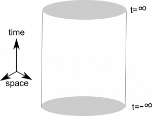
To show this, imagine spacetime as a cylinder. Each slice of the cylinder is the complete space $\mathbb{R}^3$ at a given time $t$. The lower cap of the cylinder is space at $t = – \infty$ and the upper cap space at $t = \infty$. Now, we start at $t= -\infty$ with our quantum field in a vacuum configuration with winding number zero. We have the gauge freedom to choose $A_\mu (\vec x , -\infty) =0$. (However, take note that all other pure gauge configurations, that are generated by a Gauss’ law gauge transformation are equally valid. The gauge transformations generated by Gauss’ law are those that have a gauge function in the exponent that satisfies $f(x) \to 0$ for $|x| \to \infty$. All configurations that we get from $A_\mu(\vec x , -\infty) =0$ with such a gauge transformations are also winding number zero configurations, because they are gauge equivalent to $A_\mu(\vec x , -\infty) =0$.) Each pure gauge configuration of $A_\mu$, which means $A_\mu = U^\dagger (\vec x, t)\partial U(\vec x, t) $, is a vacuum configuration. $A_\mu (\vec x , -\infty) =0$ means $U(\vec x, -\infty) =\text{const}. $
This is the naive vacuum configuration and we want to investigate what non-trivial configurations of our quantum field are possible. We are especially interested in what the final configurations at $t = \infty$ can be.
Now, remember that we work in the temporal gauge. As already mentioned above, this choice of gauge does not fix the gauge freedom completely, but instead all time-independent gauge transformations are still permitted.
In addition, we are interested in finite energy processes. This requirement means that at spatial infinity our field energy must vanish, which means that our quantum field must be in a pure gauge configuration at spatial infinity. (This is discussed in more detail in the first post).
We now put these three puzzle pieces together:
At $t = – \infty$, we have $A_\mu(\vec x , -\infty) =0$ and therefore $U(\vec x, -\infty) =\text{const}. $ At the boundary, $A_\mu$ must stay pure gauge all the way from $t= – \infty$ to $t=\infty$: $A_\mu(\infty, t) = U^\dagger (\infty, t)\partial U(\infty, t) $.
The crucial thing is now that at $t = -\infty$, we started with a configuration that corresponds to $U(\vec x, -\infty) =\text{const}$. Thus at this time, we also have at spatial infinity $U(\infty, -\infty) =\text{const}$. In the temporal gauge, only time-independent gauge transformations are permitted. Therefore, $U(\infty, -\infty) =\text{const} = U(\infty, t) = U(\infty)$ is fixed and does not change as we time moves on!
Therefore, we also have at the upper cap of the cylinder, i.e. at $t=\infty$ are pure gauge configuration (because we consider a vacuum state to vacuum state transition) $A_\mu(\infty, \infty) = U^\dagger (\infty, \infty)\partial U(\infty, \infty) $ with $U(\infty, -\infty) =\text{const}$.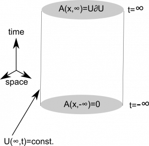
Hence, when we start with a vacuum configuration, which means a gauge transformation of $A_\mu =0$ with $U(\vec x, -\infty) =\text{const}$, our field can only transform into configurations that are gauge transformations of $A_\mu =0$ with $U(\vec x, \infty) =\text{const}$.
You may now wonder why the anything non-trivial is possible at all. The answer is that the restriction that $A_\mu$ must be pure gauge only holds:
– At the lower cap, i.e. for $A_\mu(\vec x , -\infty)$, because we start with a vacuum configuration.
– At the curved surface boundary of the cylinder, i.e. for $A_\mu(\infty, t)$, because we only consider finite energy process, which requires that the field energy vanishes at spatial infinity and thus that $A_\mu$ is pure gauge there.
– At the upper cap $A_\mu(\vec x , \infty)$, because we investigate vacuum to vacuum transitions.
Thus, in between, there is a lot of non-trivial stuff that can happen. Especially, on the way from the pure gauge at $t=-\infty$ to pure gauge $\infty$ it can be in non-pure-gauge configurations somewhere in space at some point in time. In other words, it is possible, within our restrictions that the field is, on the way from $t=-\infty$ to $t=\infty$, in a configuration that corresponds to non-zero field energy. These non-zero field energy configurations are exactly the potential barrier that we talked about in the first post. In this sense, we are dealing here with tunneling phenomena. We start with a vacuum state, i.e. zero field energy. Nevertheless, the field manages to get into configurations that “normally” would require energy to get into. However, because we are dealing with a quantum theory, it is possible that the field tunnels through these, classically forbidden configurations.
Only because this is, in principle possible, does not mean that it actually happens. However, there are solutions of the Yang-Mills equations that exactly describe such processes: the famous instanton solutions. Thus it seems reasonable that such tunneling indeed happens. (It is really cool to see how an instanton solution describes the process of how a vacuum configuration transforms into a different vacuum configuration. Different here means with a different winding number. However, there are already good descriptions in the literature and I’m currently not motivated to write down all the required formulas. An especially nice and explicit description can be found on page 168 (section 8.6.2 “Instantons as Tunneling Solutions”) in “Quarks, Leptons & Gauge Fields by Kerson Huang).
The crucial message of the description above is that we necessarily get a final field configuration that corresponds to a pure gauge configuration with $U(\vec x, \infty) =\text{const}$. The constant is necessarily the same constant that we started with at $t=-\infty$. Therefore, transitions only happen between pure gauge configurations that are generated by gauge transformations which have the same trivial limit at spatial infinity. (Trivial means that there is no dependence on angles, but instead the gauge transformation becomes the same constant no matter from which direction we approach $|x| = \infty$. )
Now, let’s connect this discussion with our previous discussion of Gauss’ law:
Recall that above we argued that the gauge transformations generated by Gauss’ law are somewhat special because we use Gauss’ law to identify physical states in a quantum theory. These gauge transformations are exactly those with a gauge function $f(x)$ in the exponent that becomes zero at spatial infinity: $U(x) = e^{if(x) \hat r \cdot \vec G}$ with $f(\infty) =0$. The naive vacuum configuration is $A_\mu=0$. All configurations that we get by transforming this configuration with a gauge transformation that is generated by Gauss’ law are completely equivalent to $A_\mu =0$, because that’s how we use Gauss’ law in a quantum theory. Therefore, starting from the naive vacuum configuration, or one that is physically equivalent, we have $U(\infty , – \infty) = 1$. Therefore, with the arguments from above, we can only end up in a configuration with $U(\infty, \infty)=1$, too!
In this sense, it is sufficient to restrict ourselves to gauge transformations that satisfy $U(x) \to 1$ for $|x| \to \infty$. This is the moral of this long story.
In my next post about the QCD vacuum, I will present another way to look at it. With this different interpretation, we can avoid all the confusing details