Although the subtle things that are often glossed over in the standard treatment of the QCD vacuum can be explained as discussed in part 2, there is another, more intuitive way to understand it.
Most importantly, this different perspective on the QCD vacuum shines a completely new light on the mysterious $\theta$ parameter.
To the expert, this perspective will be familiar. It sometimes appears in the literature and therefore the “untold” part in the headline is, of course, a bit exaggerated. However, it took me, as a student, a long long time to find it at all and most importantly a proper explanation that made sense to me.
The standard story of the QCD vacuum uses the temporal gauge. This is not a completely fixed gauge. Time-independent gauge transformations are still allowed. Only this residual gauge freedom makes the whole discussion in terms of large and small gauge transformations, etc. possible.
One may wonder what happens when we analyze the vacuum in a different gauge, where there is no residual gauge freedom. In other words: in a gauge that fixes the gauge freedom completely. Possibly choices are, for example, the axial and the Coulomb gauge.
The interpretation of the QCD vacuum is completely different in these gauges. Most importantly: there is no vacuum periodicity.
In the axial gauge, there is only one non-degenerate ground state. Then, of course, it is natural to wonder what we can learn about the $\theta$ parameter here. At a first glance, the result that there is a unique ground state implies that we have $\theta=0$. However, this is not the case and we will discuss this in a moment.
In the Coulomb gauge, there is only a non-degenerate ground state, too. However, the interpretation of the vacuum structure in this gauge is especially tricky. Most famously, one encounters the famous Gribov ambiguities. These appear because the condition that fixes the Coulomb gauge does not lead to unique gauge potentials everywhere in spacetime. Instead, there are regions where there are multiple gauge potential configurations that satisfy the condition. These configurations are called Gribov copies and the fact that we do not get a unique gauge potential configuration everywhere in spacetime is called Gribov ambiguity.
Now, how is this not a contradiction to the standard picture of the QCD vacuum? When there is only a unique non-degenerate ground state, there is no tunneling between degenerate vacua and therefore no $\theta$ parameter, right?
No! There is still tunneling and also a $\theta$ parameter. In the axial gauge, the tunneling starts from the unique ground state and ends at the same unique ground state. (In the Coulomb gauge the tunneling happens between the Gribov copies?!)
To understand this, we need an analogy.
A nice analogy to the QCD vacuum is given by the following Hamiltonian:
$$ H= – \frac{d^2 }{d x^2} + q(1-cos x) ,$$
where $-\infty \leq x \leq \infty$ and which describes a particle in a periodic potential $V(x) = q (1-cos x)$. Therefore, this situation is quite close to the standard picture of the QCD vacuum, with a periodic structure and infinitely many degenerate ground states.
Source: https://arxiv.org/abs/1505.03690
For this Hamiltonian, we have the Schrödinger equation
$$ – \frac{d^2 \psi}{d x^2} + q(1-cos x) \psi = E \psi . $$
(Among mathematicians this equation is known as the “Mathieu equation”. Sometimes it’s useful to know the name of an equation, if you want to dig deeper.)
However, exactly the same Hamiltonian describes a “quantum pendulum”. This interpretation only requires that we treat our variable as an angular variable: $x \to \phi$, with $0 \leq \phi \leq 2 \pi$ and thus
$$ – \frac{d^2 \psi}{d \phi^2} + q(1-cos \phi) \psi = E \psi . $$
Now, we identify the point $2 \pi$ with $0$ and all values of $\phi$ that are larger than $2 \pi$, with the corresponding points in the interval $0 \leq \phi \leq 2 \pi$. This implies immediately that $ \Psi(\psi + 2\pi) = \Psi(\psi) $. Therefore, the situation now looks like this:

and we no longer have infinitely many degenerate ground states, but only a unique ground state! Therefore, the situation here is exactly the same as for the QCD vacuum in a physical gauge.
Now, what about tunneling?
For a long pendulum, i.e. for large $q$, the ground state $\psi =0$ and excited states are approximately the same as for a harmonic oscillator. For large $q$, we can do a perturbative analysis in $q^{-1/2}$ and take the “anharmonicity” this way into account. However, the famously this perturbation series does not converge, because we miss something important in our analysis. Even for a pendulum with small energy, i.e. with only small perturbations around the ground state, the pendulum can “tunnel”. In this context, this means that the pendulum does a motion that it isn’t allowed to do, like rotate once around its suspension and end up again and the ground state. This is exactly what the instantons describe in a physical gauge like the axial gauge. There is no tunneling between degenerate ground states because there are no degenerate ground states. Instead, we have tunneling that starts at the unique ground state and ends again at the unique ground state. Still, this is tunneling, because there is a potential barrier that prohibits that a pendulum rotates once completely around its suspension. For a pendulum with low energy, or equally a long pendulum (large $q$), we can do the usual quantum mechanical perturbation analysis. This yields harmonic oscillator states plus small corrections from the anharmonicity. However, we must take into account that there are also quantum processes, like the tunneling once around the suspension of the pendulum.
Okay, fine. But what about $\theta$?
Well, now that we have understood that there can also be tunneling in the physical gauge picture of the QCD vacuum, which corresponds to the pendulum interpretation of the Hamiltonian in the example above, we can argue that there can be again a $\theta$ parameter. This is the phase that the pendulum picks up when it tunnels around its suspension. In a quantum theory, we can have $\Psi(\psi + 2\pi) = e^{-i \theta} \Psi(\psi) $ instead of $ \Psi(\psi + 2\pi) = \Psi(\psi) $.
When we interpret the Hamiltonian in the example above as the movement of a particle in a periodic potential, the parameter $\theta$ describes different states in the same system, completely analogous to the Bloch momenta in solid-state physics.
However, in the pendulum interpretation different $\theta$ describe different systems, i.e. different pendulums! Thus, in this second interpretation, it is much clearer why $\theta$ is a fixed parameter and not allowed to change.
To bring this point home, let’s consider an explicit example how a $\theta$ parameter can arise for the quantum pendulum.
The pendulum only picks up a phase $\theta$, when it moves in an Aharonov-Bohm potential. To make this explicit, let’s assume the pendulum carries electric charge $e$ and rotates around a solenoid with magnetic flux $\theta$. This magnetic flux is the source of a potential $ A$ in the plane of the rotating pendulum.
We get the Hamiltonian that describes this system by replacing the derivative with the covariant derivative:
$$ H= – \left(\frac{d }{d \phi} -ie A\right)^2+ q(1-cos \phi) ,$$
and thus we have the Schrödinger equation
$$ – \left(\frac{d }{d \phi} -ie A\right)^2 \psi+ q(1-cos \phi) \psi= E \psi .$$
As before, we impose the condition $ \Psi(\psi + 2\pi) = \Psi(\psi) $. However, we can also introduce a new wave function $\varphi (\psi) $ that obeys the standard Schrödinger equation without the additional vector potential
$$ – \frac{d^2 \varphi}{d \phi^2} + q(1-cos \phi) \varphi = E \varphi ,$$
where
$$ \psi(\phi) = \text{exp} \left[ ie \int_0^\phi A d\phi \right] \varphi(\phi).$$
(Take note that the relation between the magnetic flux $\theta$ and the potential $A$ is $ \int_0^{2\pi} A d\phi = \theta $).
The information about the presence of the magnetic flux and hence of the vector potential $ A$ is now, when we use $\varphi(\phi)$ instead of $\Psi (\phi)$, encoded in the boundary condition:
$$ \varphi(\phi + 2\pi) = e^{-ie\theta} \varphi(\phi). $$
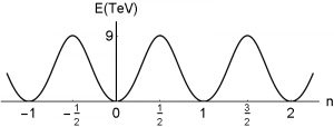
The energy of the ground state of the pendulum is directly proportional to the magnetic flux:
$$ E (\theta) \propto (1- \cos(\theta)) .$$
This show that in this model, the parameter $\theta$ defines different systems, namely quantum pendulums in the presence of different Aharonov-Bohm potentials.
In contrast, in the periodic potential picture, where $\theta$ is interpreted as analogon to the Bloch momentum, the parameter $\theta$ describes different states of the same system.
The reinterpretation of the QCD vacuum in a physical gauge with a unique non-degenerate vacuum, thus makes the appearance of $\theta$ much less obvious. This is why the standard presentation of the topic still makes use of the temporal gauge and the periodic vacuum picture.
The analysis of the QCD vacuum in the axial gauge is analogous to the interpretation of the Hamiltonian $$ H= – \frac{d^2 }{d \phi^2} + q(1-cos \phi) $$ as description of a quantum pendulum, i.e. substituting $x \to \phi$, with $0\leq \phi < 2 \pi$. (This interpretation also arises, when we work in the temporal gauge and declare that all gauge transformations (large and small) should not have any effect on the physics. The distinct degenerate vacua in the usual interpretation are connected by large gauge transformations. )
Without any further thought, one reaches immediately the conclusion that there is no $\theta$ parameter here. However, this is not correct, because a $\theta$ parameter can appear when there is an Aharonov-Bohm potential present.
When the quantum pendulum swings in such a potential, it picks up a phase when it rotates once around the thin solenoid that encloses the magnetic flux. The phase is directly proportional to the magnetic flux in the solenoid.
For the QCD vacuum, the same story goes as follows. In the axial gauge, naively there is no $\theta$ parameter because we do not have a periodic potential and hence no Bloch-momentum. However, nothing forbids that we add the term
$$ – \frac{g^2 \theta}{32\pi^2} Tr(G_{\mu\nu} \tilde{G}^{\mu\nu}),$$
where $\tilde{G}^{\mu\nu}$ is the dual field-strength-tensor: $\tilde{G}^{a,\mu \nu} = \frac{1}{2} \epsilon^{\mu \nu \rho \sigma} G^a_{ \rho \sigma}$, to the Lagrangian. This simply means that we allow for the possibility that there is an Aharonov-Bohm type potential and that it could make a difference when the pendulum rotates once around its suspension.
An obvious question is now, what the analogon to the solenoid is for the QCD vacuum. So far, I wasn’t able to find a satisfactory answer. The usual argument for the addition of $ – \frac{g^2 \theta}{32\pi^2} Tr(G_{\mu\nu} \tilde{G}^{\mu\nu})$ to the Lagrangian is that nothing forbids its existence.
So far, all experimental evidence point in the direction that there exists no “solenoid” for the QCD vacuum and therefore $\theta =0$. (The current experimental bound is $\theta < 10^{-10}$, Source).
From the analysis of the QCD vacuum in the axial gauge and by comparing it to the quantum pendulum, this does not look too surprising. However, we shouldn’t be too quick here and state $\theta =0$. Before we can say something like this, we need to understand first, what the “solenoid” could be for the QCD vacuum.
Understanding this requires that we enter a completely different world: the world of anomalies. This fascinating topic deserves its own post. Usually, it is claimed that the contribution to $\theta$ that comes from this sector of the theory is completely unrelated to the QCD $\theta$. However, we will see that anomalies and the QCD vacuum aren’t that unrelated: So far, we were only concerned with the gauge boson vacuum, while anomalies arise when we consider the fermion vacuum and its interaction with gauge bosons!
This will be discussed in part 4 of my series about the QCD vacuum.
References that describe this perspective of the QCD vacuum
- “Topology in the Weinberg-Salam theory” by N. S. Manton
- “The Interpretation of Pseudoparticles in Physical Gauges” by Claude W. Bernard, Erick J. Weinberg
- Section 11.3 in Rubakov’s “Classical Theory of Gauge Field”
- This perspective of the QCD vacuum in more abstract terms without the quantum pendulum analogy is described in “Introduction to the Yang-Mills Quantum Theory” by R. Jackiw in the around Eq. (42).