There is a deep connection between the non-trivial structure of the QCD vacuum and one of the most mysterious phenomenon in QFT: anomalies. In this part, we discuss this connection.
The thing is that, so far, we only talked about the vacuum of the gauge bosons, without saying a word about fermions. We will now see that the fermionic vacuum isn’t trivial either and that there is a close connection to what we discussed earlier for the pure gauge vacuum.
The Chiral and Axial Symmetry
If we take a look at the QCD Lagrangian with, for simplicity, just one massless quark:
$$ \mathcal{L} = -\frac{1}{4}G_a^{\mu\nu} G_{a\mu\nu} + \bar{\Psi} (i\partial_\mu \gamma^\mu -g A_\mu \gamma^\mu ) \Psi$$
we notice that there is a global symmetry
$$ \Psi \to e^{i\varphi} \Psi . $$
The conserved charge that belongs this symmetry via Noether’s theorem is simply the number of $\Psi$ particles. However, there is even more symmetry.
We can rewrite the Lagrangian in terms of left-chiral and right-chiral spinors, with the help of the usual projection operators: $\Psi_{L/R}= \frac{1}{2} (1 \pm\gamma_5) \Psi$. Then, we have
$$ \mathcal{L} = -\frac{1}{4}G_a^{\mu\nu} G_{a\mu\nu} + \bar{\Psi}_L (i\partial_\mu \gamma^\mu-e A_\mu \gamma^\mu ) \Psi_L + \bar{\Psi}_R (i\partial_\mu \gamma^\mu -eA_\mu \gamma^\mu) \Psi_R $$
and we can see that we actually have here two global symmetry:
\begin{align}
\Psi_L \to e^{i\alpha} \Psi_L \notag \\
\Psi_R \to e^{i\beta} \Psi_R
\end{align}
The corresponding Noether charges tell us that the number of left-chiral and right-chiral particles are conserved separately!
We can multiply the right-chiral and left-chiral spinors by completely different phases because there is no term here that couples left-chiral to right-chiral spinors. (Take note that a mass term couples left-chiral to right-chiral spinors and we discuss the implications of mass terms later).
At this point, you may wonder, why we care about symmetries in such an unrealistic situation. Every quark is massive and therefore we don’t actually have these symmetries! However, the masses of the two lightest quarks, the up and down quark are so tiny that they can be neglected without making a too large error. In this sense, symmetries that are present in the absence of the masses of the lightest quarks are good approximate symmetries. Such approximate symmetries are often very useful to learn something. For example, if we neglect the masses of the up quark and the down quark, we have an $SU(2)$ symmetry. This symmetry gets broken, but only a little, by the small actual masses of the up quark and the down quark. This small breaking tells us that we can expect Goldstone bosons that correspond to this breaking. Of course, because the symmetry is only an approximate one, we don’t get real massless Goldstone bosons. Yet, we get quasi-Goldstone bosons, called pions, and the approximate symmetry perspective explains why they are so light compared to all other mesons.
However, our motivation here is a bit different. Namely, we will see in a moment that even in the absence of quark masses, which would break one linear combination of these symmetries, one linear combination is broken! This anomalous breaking of the symmetries has an important implication that can actually be measured in experiments.
Now, back to our symmetries.
Noether’s theorem tells us that to each symmetry, we get a conserved current. The conserved currents here are
\begin{align}
J_L^\mu = \Psi_L \gamma_\mu \Psi_L \notag \\
J_R^\mu = \Psi_R \gamma_\mu \Psi_R
\end{align}
However, upon closer inspection, which will be discussed in a moment, it turns out that these separate currents are not conserved at all. Yet, we can find a linear combination that is conserved:
\begin{align}
J_V^\mu = J_L^\mu + J_R^\mu =\bar{\Psi} \gamma_\mu \Psi \notag \\
\partial_\mu J_V^\mu =0.
\end{align}
In turn, the orthogonal linear combination is not conserved:
\begin{align}
J_A^\mu = J_L^\mu – J_R^\mu =\bar{\Psi} \gamma_\mu \gamma_5 \Psi \notag \\
\partial_\mu J_A^\mu \neq 0.
\end{align}
The symmetry that corresponds to the conservation of $J_V^\mu$ is known as “vector $U(1)$” and denoted by $U(1)_V$. An $U(1)_V$ transformation is given by
$$ \Psi \to e^{i\phi_v} \Psi . $$
The symmetry that would exist if $J_A^\mu$ would be conserved, is known as “axial $U(1)$” and denoted by $U(1)_A$. An $U(1)_A$ transformation is given by
$$ \Psi \to e^{i \phi_a \gamma_5} \Psi . $$
The connection to the previous transformations that acted on $\Psi_L$ and $\Psi_R$ is given by $\alpha = \phi_v+\phi_a$ and $\beta = \phi_v-\phi_a$.
The situation here is similar to what happens in the standard model. There $SU(2)_L \times U(1)_Y$ gets broken to $U(1)_{em}$. The thing is that $U(1)_{em}$ is not $U(1)_Y$, but a linear combination of $U(1)_Y$ and the Cartan generator of $SU(2)_L$. Here we start with $U(1)_L \times U(1)_R$, and this symmetry “gets broken” to $U(1)_V$.
How does $U(1)_A$ get broken?
Above, we only stated that $U(1)_A$ gets broken. However, that this breaking happens is far from obvious. There is no scalar field in the theory that could be responsible for the breaking. Instead, we are dealing here with a more subtle type of symmetry breaking, called quantum mechanical symmetry breaking. A symmetry that is present in the classical theory, i.e. when we simply look at the Lagrangian, is no symmetry as soon as we use the Lagrangian in a quantum theory.
The conventional name for such quantum mechanical symmetry breaking is “anomalous breaking”.
There are several ways to see that this anomalous breaking happens.
Historically this was first discovered through a quite complicated computation of a Feynman diagram called “triangle diagram”.
The result of this computation by Adler, Bell, and Jackiw was
$$ \partial_\mu J_5^\mu = \frac{g^2}{16\pi^2} G^{\mu\nu a} \tilde{G}_{\mu \nu}^a $$
This looks shockingly like the term that we added to the Lagrangian due to the complex structure of the QCD vacuum. (This was discussed in part 4). The details regarding this laborious computation can be found in the standard textbooks, but aren’t very illuminating. Thus, we won’t go into the details here.
Instead, I want to focus on the implications and a more illustrative explanation.
Understanding the Axial Anomaly
To understand the axial anomaly, we consider the vacuum in a theory of massless fermions. To understand the theory and its vacuum, we consider its energy levels. In practice this means, we calculate the eigenmodes of the Hamiltonian.
The best picture of this vacuum is Dirac’s “sea picture”. All states with negative energy a filled up, whereas all positive energy states are empty. An electron is a positive energy state, whereas a positron is a hole in the sea of negative energy states.
In the real world, however, fermions are never alone because they carry charges. Thus, we now investigate what happens when we take the presence of gauge fields into account. We will then see that the axial anomaly is nothing but a natural consequence of the interplay between the Dirac sea and gauge fields.
To simplify the discussion, we work in two dimensions and use electromagnetic interactions, instead of the more complicated QCD interactions. The massless theory of fermions in two-dimensions, with only electromagnetic interactions present, is known as the Schwinger model. The Schwinger model is incredibly useful to understand many phenomena in quantum field theory and will prove to be invaluable here.
To simplify the discussion even further, we work in the temporal gauge: $A_0=0$. This means our gauge field has only one component $A_1 \equiv A$.
In our two-dimensional theory, we split our spinor again depending on their chirality:
$$ \Psi_+ = \begin{pmatrix} 1 & 0 \\ 0 &0 \end{pmatrix} \Psi $$
$$ \Psi_- = \begin{pmatrix} 0 & 0 \\ 0 &1 \end{pmatrix} \Psi $$
Particles with positive “chirality” are here simply particles that move to the left on our one-dimensional spatial axes (the second dimension is the time axes.) Formulated differently, positive “chirality” states are states with negative momentum. Equivalently, negative “chirality” states are states that move to the right and therefore have positive momentum.
Completely analogous to our four-dimensional problem, we can find here an anomalous divergence. Here it is proportional to $\epsilon^{\mu\nu} F_{\mu\nu} \propto \partial_t A$. We now want to answer the question: What is the origin of this anomalous divergence?
The Dirac equation for our two-dimensional model reads
$$ H \Psi_E = -\sigma_3 (\hat p – g A) \Psi_E = E\Psi_E. $$
The energy eigenstates are
\begin{align}
\Psi_+ &= \begin{pmatrix} e^{ipx} \\0 \end{pmatrix} \text{ with energy } E=-p+qA \notag \\
\Psi_- &= \begin{pmatrix} 0 \\ e^{ipx} \end{pmatrix} \text{ with energy } E=p-qA
\end{align}
Now, in the absence of the gauge field $A$, we have for the vacuum the simple Dirac sea picture outlined above. All the negative energy states are filled, while all the positive energy states are empty.
However, something interesting happens when we switch on the gauge field. As the magnitude of $A$ increases from $0$ to $\delta A$, we can see how the energy levels shift. This is best explained by a picture:
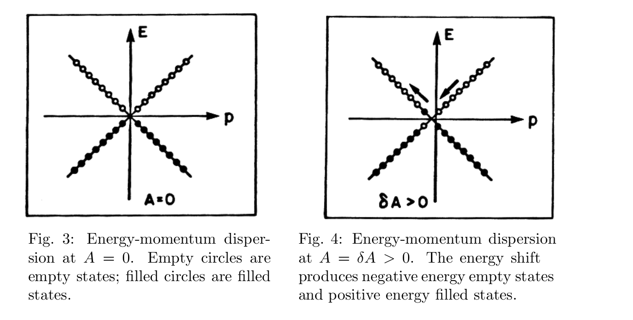
Source: https://arxiv.org/pdf/hep-th/9903255.pdf
The states with positive chirality, and hence negative momentum, do have a higher energy thanks to the gauge field $A$. In contrast, the energy levels of states with negative chirality (= positive momentum) get lower when we switch on $A$.
For the Dirac sea, this means that states that were once negative energy states and therefore filled states become now filled positive energy states. Equivalently unfilled positive energy states (= holes) now have negative energy and move below the zero energy border. In other words, the gauge field produces holes in the negative energy sea and filled positive energy states.
Let’s consider, for concreteness a positive magnitude of the gauge field $A = \delta A > 0$:
An empty state with positive momentum, positive energy, and left chirality, now acquires negative energy and therefore becomes a right-chiral antiparticle.
A filled state with negative momentum, negative energy, and right-chirality, now acquires positive energy and therefore becomes a left-chiral particle.
This means immediately that in the presence of a gauge field $A$ the charge “left-chirality” and the charge “right-chirality” are not conserved. However, the sum of “left-chirality” and “right-chirality” is still conserved! This is analogous to what we observed for the conserved current $J_L^\mu$ and $J_R^\mu$.
This is the origin of the anomaly! The gauge field produces a non-zero chirality current by lifting some states up from the Dirac sea and by pushing some holes down into the negative energy region.
It is important to take note that the shift from $A=0$ to $A= \delta A$ is a gauge transformation! The crazy thing that happens here is that such gauge transformation produces particles from the empty vacuum and this is why we get a non-zero current. What we learn here is that it is impossible to separate left-chiral and right-chiral states in a gauge invariant manner.
The fermionic vacuum, i.e. the Dirac sea, is highly susceptible to the gauge field configurations. The mere presence of the gauge fields changes the structure of the energy eigenstates and hence of the Dirac sea dramatically.
As an aside, that will be discussed in more detail in another post: This type of fermion production through gauge fields is the most popular explanation for why there is any matter at all. This explanation is known as Leptogenesis and the main idea is that topological non-trivial gauge field changes can be responsible for a nett baryon number plus lepton number surplus, while baryon minus lepton number remains unchanged.
Another important lesson here, to quote Roman Jackiw, is that:
“we must assign physical reality to Dirac’s negative energy sea, because it produces the chiral anomaly, whose effects are experimentally observed, principally in the decay of the neutral pion to two photons, but there are other physical consequences as well.”
Now, what does this mean for our axial anomaly in four dimensions?
We know that the axial current $J_5^\mu$ is anomalously non-conserved. This means that the divergence $\partial_\mu J_5^\mu$ is non-zero, and a calculation shows that it is $\propto Tr( F_{\mu\nu} \tilde{F}^{\mu\nu})$. Thus, the corresponding Noether charge
$$ Q = \int d^3 x J^0_5 $$
is not conserved. Especially, in any process where the gauge fields change such that
$$ N = \frac{1}{32 \pi^2} \int d^4x Tr( F_{\mu\nu} \tilde{F}^{\mu\nu}) \neq 0 , $$
the Noether charge $Q$ gets changed. Such a process was already discussed in the first three parts, and are commonly known as instanton and sphaleron processes. These processes change the winding number $N$. Thanks to the connection to the axial anomaly that we know now of, we understand that such processes produce a nett surplus of left-chiral and right-chiral states. Yet, the number of left-chiral minus the number of right-chiral states remains unchanged. The quantum number “left-chirality” plus “right-chirality” is not conserved and this is the breaking of the axial symmetry.
Topologically non-trivial processes like instantons and sphalerons lift fermions up from the Dirac sea and push unfilled positive states down to negative energies. This way, instantons, and sphalerons produce fermions and anti-fermion pairs.
To quote from Eric Weinberg’s book “Classical Solutions in Quantum Field Theory“:
“any change in winding number must be accompanied by a change in fermion chirality”
If you interested to learn more about this perspective on anomalies, here are a few good resources, where you can learn more:
- Chapter 9 in “An Invitation to Quantum Field Theory” by Luis Álvarez-Gaumé
- “Effects of Dirac’s Negative Energy Sea on Quantum Numbers” by R. Jackiw
- “Anomalies for pedestrians” by Barry R. Holstein
- Chapter 11 in Eric Weinberg’s book “Classical Solutions in Quantum Field Theory“
Implications of the Axial Anomaly
So, the non-conservation of the axial current $ \partial_\mu J_5^\mu \neq 0$ tells us that axial rotations $ \Psi \to e^{i \phi_a \gamma_5} \Psi $ are not a symmetry of the system. Therefore, we can now ask: How does the Lagrangian change under axial rotations?
As for anything that has to do with anomalies, there are many ways to answer this question. But, of course, the final answer is always the same:
An axial rotation $ \Psi \to e^{i \phi_a \gamma_5} \Psi $ changes our Lagrangian by
$$ \mathcal{L} \to \mathcal{L} + \frac{\alpha}{16 \pi^2} Tr[G_{\mu\nu} \tilde{G}^{\mu\nu}] . $$
Compare this to the term that we needed to add, because of the complex structure of the QCD vacuum:
$$\Delta \mathcal L = \frac{\theta}{16 \pi^2} Tr[G_{\mu\nu} \tilde{G}^{\mu\nu}]$$
It’s exactly the same!
Thus, we can say that an axial rotation by $\alpha$ shifts the mysterious $\theta$ parameter of the QCD vacuum by:
$$ \theta \to \theta + \alpha .$$
So, why does an axial rotation lead to this new term in the Lagrangian? As already mentioned above, there are different ways to see this.
1.) The standard method that is usually quoted in the textbook is known as “Fujikawa method”. (It has its own Wikipedia page). Again, I don’t want to dive into the technical details, which you can find in the standard textbooks. However, the short version is that once careful analyzes the behavior of the path integral under an axial rotation. While the Lagrangian behaves, of course, as expected from the discussion above and stays unchanged, the measure of the path integral isn’t invariant. Instead, the final result of Fujikawa’s analysis is that the change in the path integral measure due to an axial rotation amounts exactly to the change
$$ \mathcal{L} \to \mathcal{L} + \frac{\alpha}{16 \pi^2} Tr[G_{\mu\nu} \tilde{G}^{\mu\nu}] . $$
of the Lagrangian.
2.) Another way to see this is to go directly back to Noether’s theorem. (See
Palash Pal’s “An Introductory Course of Particle Physics” Eq. 4.108 at page 82 plus page 658 Eq. 21.158 or page 250 in “Classical Solutions in Quantum Field Theory” by Erick Weinberg, especially Eq. 11.57 and the text below.)
In the derivation of this theorem in the Lagrangian formalism, we calculate that when a field gets transformed
$$ \Psi^A(x) \to \Psi’^A(x)=\Psi^A(x) + \delta \Psi^A(x), $$
the change of the action is
$$ \delta S = \int d^4 x \sum_r \delta \varphi_r \partial_\mu J_r^\mu, $$
where
$$ J_r = \sum_A \frac{\partial\mathcal{L}}{\partial(\partial_\mu\Psi^A)} \frac{\partial\Psi^A}{\partial \varphi_r}$$
and $\varphi_r$ denotes a small change in a number of parameters.
(This is shown, for example at page 106 and 107 in my book “Physics from Symmetry”. In addition, take note that, as usual in the derivation of Noether’s theorem, we only consider infinitesimal transformations).
If we are dealing with a symmetry, the action does not change: $\delta S =0$ and thus we have $ \partial_\mu J_r^\mu =0$, i.e. a conserved current.
However, here we have situation where we found that $ \partial_\mu J_A^\mu \neq 0$. Thus, the corresponding transformation,an axial rotation $ \Psi \to e^{i \varphi \gamma_5} \Psi $, is not a symmetry. We can therefore conclude that the action changes under such a rotation, and the change of the action is given by
$$ \delta S = \int d^4 x \sum_R \delta \varphi_r \partial_\mu J_r^\mu . $$
In our case,
$$ \partial_\mu J_5^\mu = \frac{g^2}{16\pi^2} Tr(G^{\mu\nu a} \tilde{G}_{\mu \nu}^a )$$
and therefore, the the action changes by
$$ \delta S = \int d^4 x \, \varphi \partial_\mu J_r^\mu = \frac{g^2 \varphi }{16\pi^2} \int d^4 x \, G^{\mu\nu a} \tilde{G}_{\mu \nu}^a . $$
3.) A third method to see this change of the action, is the original method by Jackiw and Rebbi (PhysRevLett.37.172). Again, we only discuss the main idea, and do not dive into the details.
The basic idea is the following: Instead of the non-conserved current $J_5^\mu$, we define a new current that is conserved. The corresponding Noether charge generates the corresponding symmetry. Then we investigate the how this Noether charge acts on our ground state $|\theta\rangle$. The result is the same as for the previous two methods:
$$ e^{i \alpha Q_5} |\theta\rangle = |\theta + \alpha \rangle.$$
So, now let’s see how this comes about in a bit more detail.
From the discussion above, we know that $J_5^\mu = \bar{\Psi} \gamma_\mu \gamma_5 \Psi $ is not conserved. Instead, we have
$$ \partial_\mu J_5^\mu = \frac{g^2}{16\pi^2} Tr(G^{\mu\nu a} \tilde{G}_{\mu \nu}^a) . $$
Now, an important observation is, that $G^{\mu\nu a} \tilde{G}_{\mu \nu}^a$ can be written as total divergence:
$$ \frac{1}{4} G^{\mu\nu a} \tilde{G}_{\mu \nu}^a = \partial_\mu K^\mu, $$
where
$$ K^\mu = \epsilon^{\mu \alpha\beta \gamma} Tr(\frac{1}{2} A-\alpha \partial_\beta A_\gamma + \frac{i}{3} g A-\alpha A_\beta A_\gamma) $$
(A proof of this statement can be found, for example at page 89 in “Quarks, Leptons and Gauge Fields by K. Huang.)
$K_\mu$ is commonly called the Chern-Simons term or Chern-Simons current.
With the observation that $ G^{\mu\nu a} \tilde{G}_{\mu \nu}^a$ can be written as total divergence, we can define a new, actually conserved, axial current:
$$ \tilde{J}_5^\mu = J_5^\mu – \frac{g^2}{16\pi^2} K^\mu . $$
The trick here is, of course, that if we not take the divergence of this new current, the two terms simply cancel:
$$ \partial_\mu \tilde{J}_5^\mu = \partial_\mu J_5^\mu – \partial_\mu \frac{g^2}{16\pi^2} K^\mu $$
$$= \frac{g^2}{16\pi^2} Tr(G^{\mu\nu a} \tilde{G}_{\mu \nu}^a) – \frac{g^2}{16\pi^2} Tr(G^{\mu\nu a} \tilde{G}_{\mu \nu}^a) =0 . $$
The generator $Q_5$ of this $\tilde{U}(1)_A$ is, as always, the corresponding Noether charge
$$ Q_5 \equiv \int d^3x J_5^0 = \int d^3x \left[\Psi^\dagger \gamma_5 \Psi – \frac{g^2}{16\pi^2} K^0 \right]. $$
A curious feature of this Noether charge is that it isn’t gauge invariant and therefore not a physical quantity. The reason for this is that $K^\mu$ isn’t gauge invariant.
Nevertheless, we have here the generator of a symmetry and we are now interested in how the $\theta$ vacuum, that we discussed in part 4, behaves under the transformation that is generated by $Q_5$.
To do this, we employ a trick. We already saw in part 4 that if we act with some gauge transformation with winding number $n$ on our vacuum state $|\theta\rangle$, we get $ g_n |\theta\rangle = e^{in \theta}$. The idea is now, to use this to find out if $\theta$ gets changed by $Q_5$. In other words, we want to compute
$$ g_n \left( e^{i\alpha Q_5} |\theta\rangle \right) = e^{i\theta’}\left( e^{i\alpha Q_5} |\theta\rangle \right) . $$
The resulting $\theta’$ tells us how $\theta$ is affected by $e^{i\alpha Q_5}$.
To compute this, we need to know how $Q_5$ changes under gauge transformations. The result is (see Jackiw and Rebbi 1976)
$$g_n Q_5 g_n^{-1} = Q_5 + 1 .$$
With this information at hand, we can calculate
\begin{align}
g_1 \left( e^{i\alpha Q_5} |\theta\rangle \right) &= g_1 e^{i\alpha Q_5} |\theta\rangle g_1^{-1} g_1\notag \\
&= e^{i\alpha (Q_5+1)}g_1\notag \\
&= e^{i\alpha (Q_5+1)} e^{i\theta} |\theta\rangle \notag \\
&= e^{i(\theta+ \alpha)} \left( e^{i\alpha Q_5} |\theta\rangle \right) \notag \\
&\equiv e^{i\theta’} \left( e^{i\alpha Q_5} |\theta\rangle \right)
\end{align}
and thus we can conclude
$$ e^{i\alpha Q_5} |\theta\rangle = |\theta + \alpha \rangle .$$
From the discussion in part 4 we know that the existence of the non-trivial ground state $|\theta\rangle$ implies a new term in the Lagrangian
$\Delta \mathcal L = \frac{\theta}{16 \pi^2} Tr[G_{\mu\nu} \tilde{G}^{\mu\nu}].$$
The observation here that $Q_5$ shifts $\theta$, then means that the $\theta$ that appears in this new term, get shifted. Hence, we are again led to the conclusion that a chiral rotation implies a new term in the Lagrangian
$$ \Delta \mathcal L = \frac{g^2 \alpha }{16\pi^2} G^{\mu\nu a} \tilde{G}_{\mu \nu}^a$$
The Strong CP Problem
We saw in the last section that an axial rotation by $\alpha$ shifts the $\theta$ parameter of the QCD vacuum by:
$$ \theta \to \theta + \alpha .$$
Without mass terms, we can define a conserved but non-gauge invariant axial symmetry. Then we can make use of this symmetry to get rid of the parameter $\theta$. We are free to do any rotation we want and therefore, we can easily rotate $\theta$ to zero.
However, if there are mass terms
$$ m \bar \Psi \Psi = m \bar{\Psi}_L \Psi_R + m \bar{\Psi}_R \Psi_L $$
for the quarks, we no longer have this freedom. The axial symmetry is broken explicitly by the mass terms, because we are no longer free to rotate the left-chiral spinors and right-chiral spinors independently. A mass term explicitly couples a right-chiral to a left-chiral spinor. Therefore, the only allowed transformation is now
\begin{align}
\Psi_L \to e^{i\alpha} \Psi_L \notag \\
\Psi_R \to e^{i\alpha} \Psi_R
\end{align}
and
\begin{align}
\Psi_L \to e^{i\alpha} \Psi_L \notag \\
\Psi_R \to e^{-i\alpha} \Psi_R
\end{align}
is no longer a symmetry. Transforming the left-chiral and the right-chiral spinor with the same phase is a $U(1)_V$ transformation, whereas a transformation with opposite phase is an $U(1)_A$ transformation. In this sense, we can say that mass term breaks $U(1)_A$ explicitly.
Yet, we are forced to perform an axial rotation. This comes about because, in order to understand the physical content of the theory, we like to work in the mass basis where the mass matrices are real and diagonal. In general, the mass matrices aren’t real and diagonal but instead contain complex entries. The transformation
\begin{align}
\Psi_L \to U_L\Psi_L \notag \\
\Psi_R \to U_R \Psi_R,
\end{align}
where $U_L$ are unitary matrices, that make the mass matrix real and diagonal (we suppress generational indices here) leads to the emergence of the CKM matrix in the gauge sector of the theory.
A crucial observation is now that this rotation that we perform to switch to the mass basis, in general, involves an axial rotation. In particular, the desired transformation involves the rotation
\begin{align}
\Psi_L \to e^{-i ArgDet(M)} \Psi_L \notag \\
\Psi_R \to e^{i ArgDet(M)} \Psi_R .
\end{align}
(See, Eq. 191 in https://arxiv.org/pdf/hep-ph/9807516.pdf)
Thus, in contrast to the discussion of a massless theory, we are here no longer free to perform arbitrary axial rotations. Instead, there is one very special axial rotation, by the angle $\alpha = ArgDet(M)$ that we need to make the mass matrix $M$ real and diagonal.
From the discussion in the last section, we know that an axial rotation by angle $\alpha$ changes the Lagrangian
$$ \mathcal L \to \mathcal L + \frac{g^2 \alpha }{16\pi^2} G^{\mu\nu a} \tilde{G}_{\mu \nu}^a . $$
If there are mass terms, the angle $\alpha$ is fixed and given by $\alpha = ArgDet(M)$.
Thus, on the one hand, we have a parameter $\theta$ that comes from the detailed study of the QCD vacuum. On the other hand, we have a shift of this parameter through an axial rotation of quark fields by the angle $\alpha = ArgDet(M)$.
To take these two observations into account, one usually introduces a new overall parameters
$$ \bar{\theta} = \theta + ArgDet(M). $$
From experiments we know, as mentioned at the end of part 4, that $\bar{\theta}$ is tiny: $ \bar{\theta} \lesssim 10^{-9} $. Thus, in some sense the two contributions to $\bar{\theta}$ must cancel very, very precisely. This is usually called a “fine-tuning” problem, because the QCD vacuum angle $\theta$ and the $ArgDet$ must be fine-tuned to extremely high precision to yield such a tiny overall $\bar{\theta}$.
This is often presented as a big mystery. Why should there be a connection between these two seemingly completely unrelated parameters? The parameter $\theta$ was discovered by studying the pure gauge vacuum. The shift of $\theta$ by the angle $alpha$ comes from the axial rotation of fermionic fields and has its deep origin in the axial anomaly.
However, from the discussion above it should be clear that these two contributions aren’t so unrelated after all. Both originate in non-perturbative processes like instantons.
The emergence of $\theta$ as a parameter that describes the QCD vacuum structure, was a result of instanton process. In the temporal gauge, we discovered
An unrealistic solution of the strong CP problem
One trivial solution to the strong CP problem was, in principle, already mentioned above. Without a mass term $\bar{\theta}$ wouldn’t be a physical parameter because we can give it any term we want through axial rotations. However, if there is a mass term, we no longer have this freedom.
In the real world, there are many quarks and therefore, in the absence of mass terms many axial symmetries: one for each quark. This means immediately that when one quark is massless, say the up-quark, we could perform an arbitrary axial rotation of the corresponding spinors. Following the discussion above, this would immediately mean that $\theta$ is not a physical quantity because we can change it at will via this axial rotation.
Only, if all fermions do have mass, $\bar{\theta}$ is a physical parameter. However, as far as we know this is actually the case and therefore $\bar{\theta}$ physical. Yet, “one massless quark” is commonly quoted as a solution of the strong CP problem.