We have already discussed why the gauge couplings depend on the energy scale and how we can compute the renormalization group equations (RGEs) that describe how the couplings change with energy. In this post we talk about how we can solve the RGEs.
The Standard Model RGEs
To solve the RGEs, we need boundary conditions. One such condition is always given by the measured values of the coupling constants. Usually we use the couplings strength at the energy scale that is given by the mass of the $Z$-boson:
\begin{align}
\omega_{1Y}(M_Z)& = 59.0116 \, ,\notag \\
\omega_{2L}(M_Z)& = 29.5874 \, , \notag\\
\omega_{3C}(M_Z)& = 8.4388 \, , \notag \\
M_Z &= 91.1876 \text{ GeV} \, ,
\end{align}
These values are taken from the Review of Particle Physics.
Then, using the general formula described in this post, we can derive the RGEs, for example, for the standard model gauge couplings. The Standard Model RGE coefficients are
\begin{align}
a_{SM}=\left(
\begin{array}{c}
\frac{41}{10} \\ -\frac{19}{6} \\ -7
\end{array}
\right) \qquad , \qquad
b_{SM}= \left(
\begin{array}{ccc}
\frac{199}{50} & \frac{27}{10} & \frac{44}{5} \\
\frac{9}{10} & \frac{35}{6} & 12 \\
\frac{11}{10} & \frac{9}{2} & -26 \\
\end{array}
\right)
\end{align}
and putting them into Equation 2 of this post yields differential equations that can be solved, for example, using Mathematica.
The solutions of the $2$-loop RGEs for the Standard Model gauge couplings are shown in the figure below.
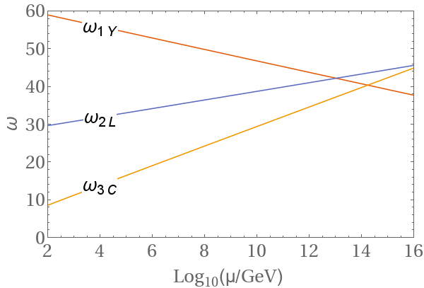
We can see that the couplings do not meet exactly at one point. This is famous result that in non-supersymmetric GUTs one needs at least one intermediate scale or additional particles to achieve the unification of the gauge couplings.
Before we can solve the RGEs with an intermediate scale, we need to discuss the matching conditions at the various scales.
Matching Conditions
As a first approximation, we can compute the unification scale by determining where the gauge couplings meet at one point. This would mean, for example, that we use the boundary condition
\begin{equation} \omega_{1Y}(M_{GUT}) = \omega_{2L}(M_{GUT})= \omega_{3C}(M_{GUT}) \end{equation}
In this first approximation $M_{GUT}$ is the scale where the heavy vector bosons and scalars get integrated out. At scales far above this mass scale, the spontaneous symmetry breaking has a negligible effect. This procedure is sufficient when we use the $1$-loop RGEs.
Unfortunately, if we want to determine the GUT scale with higher accuracy and use the $2$-loop RGEs, this picture is vastly oversimplified. It is unlikely that all vector bosons and scalars have exactly the same mass. If their masses are not degenerate the correct matching conditions for a breaking $G \rightarrow \prod_i G_i$ are
\begin{equation}
\label{eq:thresholddef}
\omega_{G_i}=\omega_{G}-\frac{\lambda_i(\mu)}{12 \pi} ,
\end{equation}
where
\begin{eqnarray}
\label{eq:lambdasthresholds}
\lambda_i(\mu)= \underbrace{\left( C_2(A_G)-C_2(A_i) \right)}_{\lambda_i^G} -21 \underbrace{ \; T(V)\ln \frac{M_V}{\mu}}_{\lambda_i^V} + \underbrace{T(S) \ln \frac{M_S}{\mu}}_{\lambda_i^S} + 8 \underbrace{T(F) \ln \frac{M_F}{\mu} }_{\lambda_i^F} \, .
\end{eqnarray}
Here $V$, $S$ and $F$ denote the vector, scalar and fermion subgroup representations that get integrated out at the matching scale $\mu$ and $M_V$, $M_S$, $M_F$ their masses. Once more $C_2(r)$ and $T(r)$ denote the quadratic Casimir invariant and the Dynkin index of the representation $r$. Further, $A_G$ and $A_i$ denote the adjoint representation of the group $G$ and subgroup $i$. In words this means the GUT scale is no longer where the gauge coupling meet at one point, but can lie above or below this point.
For the moment, we neglect the logarithmic terms and discuss them in a later post. Initially it was assumed that the logarithmic terms are small and therefore negligibly. However, in GUTs there are ususually lots of scalar fields and altough the contribution from each individual scalar field is small, many small contributions can add up to a large term. The corrections coming from these logarithmic terms are usually called threshold corrections.
Without the logarithmic terms, we can derive, for example, for the breaking chain ${SO(10) \rightarrow SU(4) \times SU(2)_L \times SU(2)_R \rightarrow \text{SM}}$ the following matching conditions at the $SO(10)$ scale
\begin{align} \label{eq:so10matching}
\omega_{SU(4)_C}(\mu_u) – \frac{4}{12\pi}&= \omega_{SO(10)}(\mu_u) – \frac{8}{12\pi} \, , \notag \\
\omega_{SU(2)_L}(\mu_u) – \frac{2}{12\pi}&= \omega_{SO(10)}(\mu_u) – \frac{8}{12\pi} \, , \notag \\
\omega_{SU(2)_R}(\mu_u) – \frac{2}{12\pi} &= \omega_{SO(10)}(\mu_u) – \frac{8}{12\pi}
\end{align}
\begin{align} \label{eq:patiso10matching}
\omega_{SU(3)_C}(\mu_i) – \frac{3}{12\pi}&= \omega_{SU(4)_C}(\mu_i) – \frac{4}{12\pi} \, , \notag \\
\omega_{SU(2)_L}(\mu_i) – \frac{2}{12\pi} &= \omega_{SU(2)_L}(\mu_i) – \frac{2}{12\pi} \, , \notag \\
\omega_{U(1)_Y}(\mu_i) &= \frac{3}{5}\left( \omega_{SU(2)_R}(\mu_i) – \frac{2}{12\pi} \right) + \frac{2}{5}\left( \omega_{SU(4)_C}(\mu_i) – \frac{4}{12\pi} \right) \, .
\end{align}
To derive these, we have simply used Eq. \ref{eq:lambdasthresholds} and the numerical values for the quadratic Casimirs, which are listed, for example, in the last section of this post.
The RGEs in Models with enlarged Gauge Symmetry
Now equipped with these matching conditions, we can finally solve the RGEs in an $SO(10)$ model with a Pati-Salam intermediate symmetry. We use the coefficients computed in this post for the running between the Pati-Salam and the $SO(10)$ scale:
\begin{align} \label{eq:paticoefficients}
a_{PS} = \left(
\begin{array}{c}
\frac{26}{3} \\ \frac{26}{3} \\ \frac{2}{3}
\end{array}
\right) \, , \qquad
b_{PS}= \left(
\begin{array}{ccc}
\frac{779}{3} & 48 & \frac{1277}{2} \\
48 & \frac{779}{3} & \frac{1277}{2} \\
\frac{249}{2} & \frac{249}{2} & \frac{3541}{6} \\
\end{array}
\right).
\end{align}
The Standard Model RGEs are unchanged and therefore as described in the first section. Using the matching conditions from above, we can solve the RGEs, for example, using Mathematica. The result is shown in the following figure.
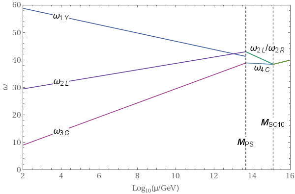
We can see that through the intermediate symmetry we can achieve unifcation of the gauge couplings. This is possible, because we now have one additional fit paramter: the intermediate scale $M_{PS}$.
This breaking chain was thought to be ruled out, because the $SO(10)$ scale is quite low and therefore the proton lifetime is below the present bound from the Super Kamiokande experiment. However as already mentioned above, there can be large threshold corrections, when not all scalar particles that get integrated out at a given scale habe exactly the same mass. Therefore this breaking chain was recently reanalysed in this paper. The authors found that the proton lifetime can be well above the present bound from Super Kamiokande through the threshold corrections.