If you understand the idea Lie Group= Manifold, you can easily understand one of the most curious facts of Lie theory:
The Lie algebra g, which is defined as the tangent space at the identity TeG, is able to tell us almost everything about a given Lie group G.
The connection between Lie algebra elements and Lie group elements is established by the exponential map. We can understand this easily from the “naive”, historical approach to Lie theory that deals with infitesimal transformations. The differential geometry perspective enables us to understand this connection in a more pictorial way.
There are four simple concepts one needs to know in order to understand the connection between Lie algebra elements and Lie group elements: Curves, Functions, Vector Fields, and Integral Curves.
Curves:

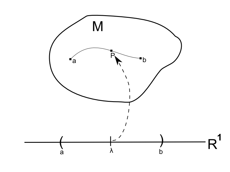
Illsutration of a curve on M, as a map from R1 onto M. The point λ of R1 is mapped onto P in M.
One way to think about a curve on a manifold M is as continuous series of points in M. The definition we want to use is, that a curve is a mapping from an open set of R1 into M. Therefore, a curve associates with each point λ of R1 (which is just a real number) a point in M. The curved is said to be parametrized by λ. The point in M is called the image point of λ. Two curves can be different even though they have the same image points in M, if they assign a different parameter value to the image points.
Functions:

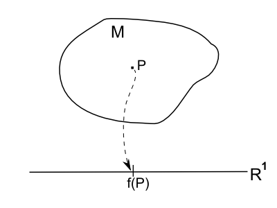
Illustration of a function on a manifold as map from M onto R1
Functions are in some sense inverse to curves. A function on a manifold M assigns a real number (= a element of R1) to each point of M. To make sense of the word differentiable when talking about functions on M, it helps to think about differentiability in terms of coordinates.
Remember that a manifold is defined as a set for which in the neighborhood of any point a map onto Rn exists. In other words: We can assign in the neighborhood of any point coordinate values to the points in the neighborhood. Therefore we can combine this map onto Rn, with the map (function) from M to R1 to get a map from Rn onto R1. A function is said to be differentiable if the it is differentiable in Rn.
In the abstract sense a function is a map f(P), where P denotes some point in M. By assigning coordinate values to this point, we have a map f(x1,x2,…,xn). If this function is differentiable in its arguments, the function is said to be differentiable. The coordinate map itself gives us a function for each coordinate. For example x2(P) is a function that maps each point P to the corresponding coordinate value x2.
Tangent Vectors:
Now we head to something that is quite hard to grasp when stumbling about it for the first time: The modern, abstract definition of a tangent vector.
We start with a curve that passes through some point P of M. This curve is described, using the coordinate map, by the equations xi(λ). A differentiable function f=f(x1,x2,…,xn), abbreviated f=f(xi), on M assigns a value to each point of the curve. To be precise we call this function, g(λ), because f is a function of (x1,x2,…,xn) and g is a function of λ.
g(λ)=f(x1(λ),x2(λ),…,xn(λ))=f(xi(λ))
We can differentiate, which yields, using the chain rule
dgdλ=∑idxidλδfδxi.
Because this equation holds for any function f, we can write
ddλ=∑idxidλδδxi.
(If this seems strange to you, you may check out chapter 8.1 of the Feynman Lectures about Quantum Mechanics, which has a great explanation regarding this, “removing objects from an equation, if it holds for arbitrary objects of this kind)
If we would be talking exclusively about Euclidean space, we would interpret dxidλ as the components of a vector tangent to the curve. dxi are infinitesimal displacement along the curve by dividing them by a real number λ, gives the rate of change in this direction. Dividing by a real number does only change the scale, not the direction of the displacement.
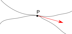
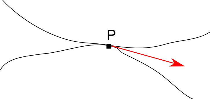
Illustration of two different curves having the same tangent vector at some point P
Every curve has a unique tangent vector at any point. In contrast a tangent vector can be the tangent vector for infinitely many curves. For example, if we take a look at the simple curve
xi(λ)=λai
with constants ai. The tangent vector at the point P, λ=0 is dxidλ=ai. A slightly different curve
xi(μ)=μ2bi+μai
goes through the same point P for μ=0 and has the same tangent vector at P, dxidμ=ai.

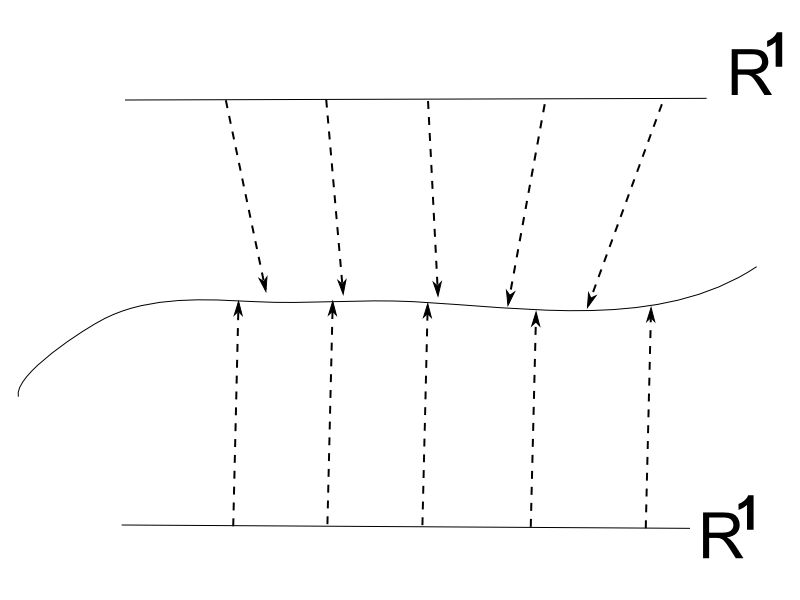
Illustration of two curves having the same path but different parameterizations.
Furthermore, we can reparametrize the first curve by xi(ν)=(ν3+ν)ai. This curve goes through the same points, but has different values ν associated with them. At ν=0, this curve goes again through P and the tangent vector is dxidν=ai.
We conclude: Every vector belongs to a whole equivalence classes of curves at this point. More dramatically one can say: The vector characterizes a whole equivalence classes of curves at this point. The defining feature of this equivalence class is the vector.
This observation motivates the modern definition of a tangent vector. In Euclidean space we have no problem with talking about displacements. A vector in Euclidean space points from one point to another. On a manifold there is, in general, no distance relation between points. Therefore, we need a more sophisticated idea to be able to talk about vectors.
Consider a curve xi=xi(μ) through P. Analogous to the considerations above we have
ddμ=∑idxidμδδxi.
Using two numbers a and b, we can take a look at the linear combination
addλ+bddμ=∑i(adxidλ+bdxidμ)δδxi.
adxidλ+bdxidμ are components of a new vector that is tangent to some curves through P. Therefore, for one of these curves that is parametrized by Φ, we can write at P
ddΦ=∑i(adxidλ+bdxidμ)δδxi.
and therefore
ddΦ=addλ+bddμ.
At this point we can see that we have a one-to-one correspondence between the space of all tangent vectors at some point P and the space of all derivatives along curves at P.
The directional derivatives, like ddλ, behave like the usual vectors under addition and are therefore said to form a vector space. A basis for this vector space is always given by {δδxi}, because we have seen that any directional derivative can be written as a linear combination of the derivatives δδxi, the derivatives along the coordinate lines. The components in this basis are {dxidλ}.
The definition of a tangent vector that mathematicians prefer is that ddλ is the tangent vector to the curve xi(λ). This definition is advantageous, because it involves no displacements over finite separations and it makes reference to coordinates. The definition makes sense, because, as we can see above, ddλ has the components {dxidλ}, if we pick some coordinate system, which are exactly the numbers one associates naively with an “arrow” tangent to a curve.
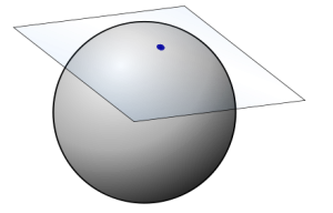
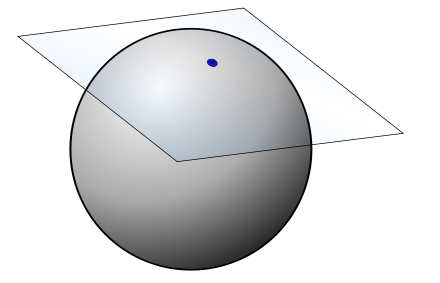
Illustration of the tangent space for some point on the sphere
The subtle point is that we are no longer allowed to add vectors located at different points of the manifold. The vectors are said to live in the tangent space of M at P, denoted TPM. Therefore vectors at different points live in different spaces and are not allowed to be added together. Using the sphere as an example, one may picture this tangent space as a plane lying tangent to the sphere this point.
Vector Fields and Integral Curves
Another important term is vector field. A vector field is a rule that defines a vector at each point of the manifold. We have one tangent space at each point of the manifold and a vector field is a rule that picks one vector from each tangent space. As already noted above: Every curve has at each point a tangent vector. We can turn this a bit upside-down. Given a vector field, i.e. a tangent vector at each point of the manifold, we can find, if we pick one point P, precisely one curve going through P that has exactly the tangent vector the vector field picks as a tangent vector at any point the curves passes through. Such a curve is called a integral curve, because given a vector field Vi(P), in coordinates Vi(P)=vi(xj), the statement that these vectors are tangent vectors to curves is mathematically
dxidλ=vi(xj).
This is just a first order differential equation for xi(λ) that has always a unique solution in some neighborhood of P.
The Exponential Function on a Manifold
We are now in the position to understand the tool that connects Lie algebra elements and Lie group elements: The exponential function. Given a vector field Y=ddλ, we can find the corresponding integral curve xi(λ) through some point. The coordinates of two points (λ0 and λ0+ϵ) on this curve are related by the Taylor series
xi(λ0+ϵ)=xi(λ0)+ϵ(dxidλ)λ0+12!ϵ2(d2xidλ2)λ0+…=(1+ϵddλ+12!ϵ2d2dλ2+…)xi|λ0=exp(ϵddλ)xi|λ0
The exp notation here should be understood as a shorthand notation for series of differential operators that act on xi, evaluated at λ0.
The Lie algebra
The Lie algebra is defined as the tangent space at the identity TeG, of the manifold G. We will now see that each element of TeG, i.e., each tangent vector at the identity defines a unique vector field V on G.
We can then find the corresponding integral curve for this vector field V that goes through e and has tangent vector Ve at the identity. By using the exp operator, as defined above, we can get to any point on this curve. V is completely determined by Ve and therefore the points of G on this curve can be denoted by
gve(t)=exptV|e
This is how we are able to get Lie group elements from Lie algebra elements. We have a one-to-one correspondence between tangent vectors and differential operators and are therefore able to use the exp notation to describe the corresponding Taylor series. This Taylor series connects different points on the same curve and therefore we are able to get from each element of the Lie algebra TeG, elements of the Lie group G.
We will now take a look at how each tangent vector at the identity defines a unique vector field.
The Lie algebra and left-invariant vector fields
Given a Lie group G, natural maps (diffeomorphisms) are left- and right-translations. That is any element g of G defines a map from a point h of the manifold G onto some new point gh (left-translation) or hg (right-translation).
h→gh left−translationorh→hg right−translation
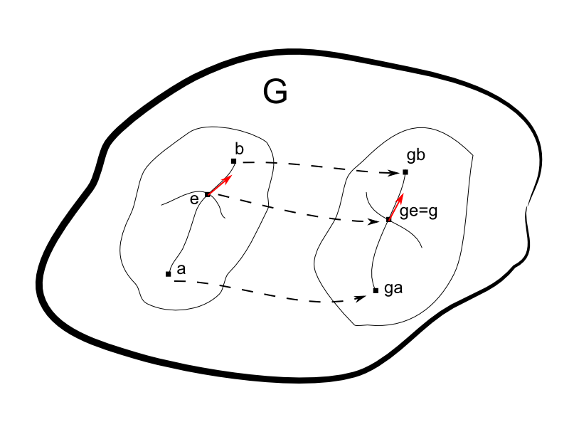
Left translations along g, map a neighborhood of e onto a neighborhood of g. In addition curves through e are mapped onto curves through g, and therefore tangent vectors at e onto tangent vectors at g
Here the group acts on itself. Of course we are able to examine how a group acts on different manifolds, too, and this idea is investigated further by representation theory. For now it suffices to have a look at these maps of G onto itself.
Everything that follows can be done with right-translations, but its convention to use left-translations.
As always we denote the identity element of the group by e. The left-translation map along a particular g, maps any neighborhood of e onto a neighborhood of g (See the figue below). In addition, this map, maps curves into curves and therefore tangent vectors into tangent vectors.
The map between tangent vectors is commonly denoted Lg:Te→Tg. A vector field V is said to be left-invariant if Lg maps V at e to V at g (and not to some different vector field at g, for example, some W), for all g. Because of the group composition law this is equivalent to saying that a vector field is left-invariant if Lg maps V at h to V at gh, for any h.
Every vector in Te defines a left-invariant vector field. The rule for getting a vector at each point of the manifold is given by Lg. By multiplication with some g∈G, we get from any vector in TeG a vector in TgG, and by definition this is what we call a left-invariant vector field.
Therefore, the set of left-invariant vector fields is isomorphic to the elements of TeG, i.e., the Lie algebra of G. Mathematicians say the set of left-invariant vector fields is the Lie algebra of G. ( The defining feature of a Lie algebra, the Lie bracket can be easily proved using coordinates. One needs to show that Lg maps [V,W] at e into [V,W] at g, which means the vector field [V,W] is again left-invariant. )
The distinction is necessary, because of the abstract definition of a Lie algebra. The set of all vector fields on G form a Lie algebra, too, but this is not the Lie algebra one has normally in mind when talking about the Lie algebra of a given Lie group.
Summary
In the last section we saw, how each element of TeG defines uniquely a vector field on G. Each element of the Lie algebra can be identified with a left-invariant vector field.
To each left-invariant vector field, and therefore to each element of TeG belongs one unique integral curve through the identity element e of G. We can get to points on this curve, by using the exponential map, which is shorthand for the Taylor series
gve(t)=exp(tV)|e.
Starting with a different element of TeG we have a different integral curve and are able to reach different points of G. (This does not hold in general. Two different elements of TeG, would be v and 2v. The corresponding integral curves go through the same points of G, only the “speed” (parameter value) differs. Nevertheless, for some elements we can get to different points)
This is how the Lie algebra TeG of group G is able to describe to describe the group G.
 Update 10.4.16: