Lie Group Theory – A Completely Naive Introduction

In this posts we discuss how continuous symmetries can be described mathematically. Many important features of such symmetries can be described using something simple, called Lie algebras. In the second part of this post you will see why a new object, called Lie bracket, is the defining feature of a Lie algebra.

As an aside: Group theory is the branch of mathematics one uses to work with symmetries. If you don’t know already what group theory is all about, have a look at my my post about it.

The branch of Group theory that deals with continuous symmetries is called Lie theory. This means that Lie groups have elements which are arbitrary close to the identity transformation. (The identity transformation is the transformation that changes nothing at all.)

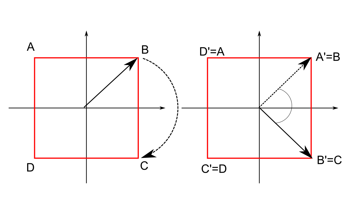
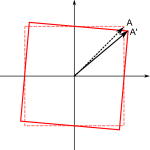
An arbitrary group has, in general, no element close to the identity. Take for example the symmetries of a square. The set of transformations that leave the square invariant are four rotations: a rotation by 0°, by 90°´, by 180° and one by 270°, plus some mirror symmetries. A rotation by 0,000001°, which is very close to the identity transformation (a rotation by 0°), is not in the set of transformations.

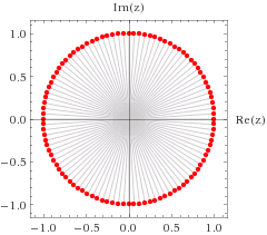
Next, take a look at the symmetry transformations of a circle. Certainly, a rotation by 0,000001° is a symmetry of the circle. One says, the symmetry group of a circle is continuous, because the rotation parameter (the rotation angle) can take on arbitrary (continuous) values. Mathematically, with the identity denoted $I$, an element $g$ close to the identity is denoted \begin{equation} g(\epsilon)=I+ \epsilon X \end{equation} where the $\epsilon$ is, as always in mathematics, some really, really small number and $X$ is an object, called generator, we will talk about in a moment.

Such small transformations, when acting on some object change barely anything. In the smallest possible case, such transformations are called infinitesimal transformation. Nevertheless, repeating such an infinitesimal transformation often enough, results in a finite transformation. Think about rotations: Many small rotations in one direction is equivalent to one big rotation in the same direction.

Mathematically, we can write the idea of repeating a small transformation many times \begin{equation} h(\theta)=(I+ \epsilon X) (I+ \epsilon X) (I+ \epsilon X) … = (I+ \epsilon X) ^k, \end{equation} where $k$ denotes how often we repeat the small transformation.

If $\theta$ denotes some finite transformation parameter, e.q. 50° or so, and $N$ is some really big number that makes sure we are close to the identity, we can write the term above as \begin{equation} g(\theta)=I+ \frac{\theta}{N} X \end{equation} The transformations we want to consider are the smallest possible, which means $N$ must be the biggest possible number, i.e. $N \rightarrow \infty $. To get a finite transformation from such a infinitesimal transformation, one has to repeat the infinitesimal transformation infinitly often. Mathematically \begin{equation} g(\theta)= \lim_{N \rightarrow \infty} (I+ \frac{\theta}{N} X) ^N \end{equation} which is in the limit just the exponential function \begin{equation} g(\theta)= \lim_{N \rightarrow \infty} (I+ \frac{\theta}{N} X) ^N = e^{\theta X} \end{equation} In some sense the object $X$ generates the finite transformation $g$, which is why its called the generator. This will be made more precise in a moment, but first take a look at another way of looking at this:

If we are considering a continuous group of transformations that are given by matrices, we can make a Taylor expansion of an element of the group around the identity, as long as the element is close to the identity, which means the transformation parameter $\theta$ is small. For a big transformation parameter $\theta$, which means a bigger transformation the first terms of the Taylor series aren’t a good approximation for the transformation. The Taylor series is \begin{equation} g(\theta)=I+ \frac{ dg}{d \theta }. |_{\theta=0} \theta + \frac{ d^2g}{d \theta^2 }. |_{\theta=0} \theta^2 + … = \sum_n \frac{d^n g }{d \theta^n }\big{|}_{\theta=0 } \theta^n \end{equation} This series expansion can be written in a more compact form, remembering the series expansion of the exponential series \begin{equation} g(\theta)= e ^{ \frac{ dg}{d \theta }. |_{\theta=0} \theta } \equiv \sum_n \frac{d^n g }{d \theta^n }\big{|}_{\theta=0 } \theta^n. \end{equation} and we can see now, how to make the connection to the previous description. By comparision with the result above: $ X = \frac{ dg}{d \theta }. |_{\theta=0} $

The idea behind such lines of thought is, that one can learn a lot about a group by looking at the important part of the infinitesimal elements (denoted $X$ above): the generators.

In the following posts, using the language of differential geometry, the reason for why this is possible and how it makes things much easier, will be explained in great detail.

For matrix Lie groups one defines the Lie algebra corresponding to the Lie group as the collection of objects that give an element of the group when exponentiated. (This is an easy definition one can use when restricting to matrix Lie groups. Later we will introduce a more general definition.)

In mathematical terms:

For a Lie Group $G$ (given by a $n\times n$ matrix), the Lie algebra $\frak{g}$ of $G$ is given by those $n\times n $ matrices $X$ such that $e^{tX} \in G$ for $t \in R$.

We know from the definition of a group that a group is more than just a collection of transformations: The definition of a group includes a binary operation $\circ$ for combining transformations. For matrix Lie groups this is just ordinary matrix multiplication. Naivly one may think that the same combination rule $\circ$ is valid for elements of the Lie algebra. This is not the case! The elements of the Lie algebra are given by matrices (a famous theorem of Lie group theory, called Ado’s Theorem, states that every Lie algebra is isomorph to a matrix Lie algebra.), but the multiplication of two matrices of the Lie algebra doesn’t has to be an element of the Lie algebra. Instead, there is another combination rule for the Lie algebra that is directly connected to the combination rule of the corresponding Lie group.

The connection between the combination rule of the Lie group and the combination rule of the Lie algebra is given by the famous Baker-Campbell-Hausdorff-Formula:

\begin{equation} \mathrm{e}^{X} \circ \mathrm{e}^{Y} = \mathrm{e}^{X+Y+\frac{1}{2}[X,Y]+\frac{1}{12}[X,[X,Y]]-\frac{1}{12}[Y,[X,Y]]+\ldots} \end{equation}

On the left hand side, we have the multiplication of two elements of the Lie group, lets name them $g$ and $h$, which we can write in terms of the corresponding generators:

\begin{equation} gh= \mathrm{e}^{X} \circ \mathrm{e}^{Y} \end{equation}

On the right-hand side we have a single object of the group $\mathrm{e}^{X+Y+\frac{1}{2}[X,Y]+\frac{1}{12}[X,[X,Y]]+\ldots} $ and the multiplication of the group elements have been translated to a sum of Lie algebra elements. The new symbol appearing in this sum $[,]$ is called Lie bracket and for matrix Lie groups it is given by $[X,Y]=XY-YX$, which is called the commutator of $X$ and $Y$.The elements $XY$ and $YX$ need not to be part of the Lie algebra, but their difference always is!

We learn from the Baker-Campbell-Hausdorff-Formula that the natural product of the Lie algebra is , not as one would naivly think, ordinary matrix multiplication, but the Lie bracket $[,]$. One says, the Lie algebra is closed under the Lie bracket, just as the group is closed under the corresponding composition rule $\circ$, e.q. matrix multiplication.

The abstract definiton of a Lie algebra will use the Lie bracket as the defining object. A Lie algebra is defined by its Lie bracket. As always, things become much easier when we look at some examples.

Example: Rotations in three dimensions and the group SO(3)

We start with rotations in three dimensions. The defining feature of a rotation is that it leaves the length of any vector unchanged. The length of a vector in three-dimensions is given by the standard scalar-product of the vector with itself

$ length = \vec v\cdot \vec v = \vec v^T \vec v,$

where the upper $T$ denotes transposing. We exchanged the scalar product $\cdot$ by ordinary matrix (a three dimensional vector is then just a (1,3) matrix) multiplication, which requires that we transpose (exchanging columns and lines of a matrix) the vector to the left, to get the same result that we get using the rules of the scalar product. In what ways can we transform the arbitrary vector $\vec v $ such that its length remains unchanged? We denote the transformation by a matrix $O$ and therefore $v’=O \vec v$. The length of this transformed vector is

$ length’ = \vec v’\cdot \vec v’ = \vec v’^T \vec v’ = \vec v ^T O^T O \vec v,$ (using that for two matrices $A$ and $B$, $(AB)^T= B^T A^T$ holds)

and requiring that the matrix $O$ doesn’t change the length of the vector means

$ length’ = length \rightarrow \vec v’^T \vec v’= \vec v^T \vec v \rightarrow \vec v ^T O^T O \vec v = \vec v^T \vec v$

and therefore $O^T O =1$ must hold. This is defining condition of a matrix Lie group, called $O(3)$, where the $O$ stands for orthogonal and $3$ for 3 dimensions.

Unfortunately, leaving length unchanged is not an exclusive feature of rotations. Mirror transformations have this property, too. Nevertheless, rotations preserve the orientation (right-handed coordinate system $\rightarrow$ right-handed coordinate system) , whereas mirror transformations change it, by definition (right-handed coordinate system $\rightarrow$ left-handed coordinate system). Therefore we restrict the transformation to rotations if we demand $\det(O)=1$. (This is a basic result of linear algebra, you can read about for example at Wikipedia if you don’t know already about it.)

Therefore, all $3\times3$ matrices fulfilling the two condition $O^T O =1$ and $\det(O)=1$ describe rotations in three dimensions. These two conditions define a matrix Lie group called $SO(3)$, where $O$ stands for orthogonal ($O^T O =1$) and $S$ for special ($\det(O)=1$ ). A basis for this group are the usual rotation matrices in three dimensions. (You can check that these matrices fulfil the defining conditions and that they are linearly independent.)

\begin{equation} R_x= \begin{pmatrix}
1&0 &0 \\ 0&\cos(\theta) &- \sin(\theta) \\ 0 & \sin(\theta)& \cos(\theta)
\end{pmatrix} \qquad R_y= \begin{pmatrix}
\cos(\theta)&0 &-\sin(\theta) \\ 0& 1 & 0 \\ \sin(\theta)& 0& \cos(\theta)
\end{pmatrix} \end{equation}

\begin{equation} R_z= \begin{pmatrix}
\cos(\theta)& \sin(\theta) &0 \\ -\sin(\theta) &\cos(\theta) & 0 \\ 0 & 0& 1
\end{pmatrix} \end{equation}

For example, if we want to rotate the vector
\begin{equation} \vec v = \begin{pmatrix} 1 \\ 0 \\ 0 \end{pmatrix}
\end{equation} around the z-axis, we multiply it with the corresponding rotation matrix
\begin{equation} R_z(\theta) \vec v = \begin{pmatrix}
\cos(\theta)& \sin(\theta) &0 \\ -\sin(\theta) &\cos(\theta) & 0 \\ 0 & 0& 1
\end{pmatrix} \begin{pmatrix} 1 \\ 0 \\ 0 \end{pmatrix} = \begin{pmatrix} \cos(\theta) \\-\sin(\theta) \\ 0 \end{pmatrix} \end{equation}

Lie algebra of SO(3)

We can now derive the Lie algebras of $SO(3)$. The definition given in the last section for the Lie algebra was that its the set of matrices that gives elements of the group by exponentiation.

The defining conditions for the $SO(3)$ group are

\begin{equation} \label{eq:defSO3} O^T O \stackrel{!}{=} I \qquad {\mathrm{ and }} \qquad \det(O)\stackrel{!}{=}1\end{equation}

Consider an infinitesimal transformation

\begin{equation} O_{\mathrm{inf }} = I+ \epsilon J,\end{equation}

where we get a finite transformation as usual by exponentiating. Putting this into the first defining condition we get

\begin{equation}( I+ \epsilon J)^T (I+ \epsilon J)=I \qquad \rightarrow \qquad I + \epsilon J^T + \epsilon J + \underbrace{\epsilon^2 J^T J}_{\approx 0 \text{ because } \epsilon^2\approx0} = I \end{equation}

\begin{equation} \label{eq:bed1} \rightarrow J^T + J \stackrel{!}{=}0 \end{equation}
A user named assjtt at reddit pointed out correctly that $J^T + J \stackrel{!}{=}0$ already implies $tr(J) = 0$ and therefore the following lines aren’t necessary to derive this.

Using the second condition and the identity $\det({\mathrm{e }}^{A})= {\mathrm{e }}^{{\mathrm{tr }}(A)}$ for the matrix exponential function, we see

\begin{equation} \det(O) \stackrel{!}{=} 1 \qquad \rightarrow \qquad \det({\mathrm{e }}^{\Phi J}) = \mathrm{e }^{\Phi{\mathrm{tr }}(J)} \stackrel{!}{=} 1
\end{equation}

\begin{equation} \label{eq:bed2} \rightarrow {\mathrm{tr }}(J) \stackrel{!}{=} 0 \end{equation}

Three linear independent (therefore these matrices are a basis of all 3×3 matrices fulfilling these conditions, from which all other can be constructed by linear combinations.) matrices fulfilling the conditions eq.\ref{eq:bed1} and eq.\ref{eq:bed2} are

\begin{equation} \label{eq:SO3-generators} J_1= \begin{pmatrix}
0&0 &0 \\ 0&0 & -1 \\ 0 & 1& 0
\end{pmatrix} \qquad J_2= \begin{pmatrix}
0&0 &1 \\ 0&0 & 0 \\ -1 & 0& 0
\end{pmatrix} \qquad J_3= \begin{pmatrix}
0&-1 &0 \\ 1&0 & 0 \\ 0 & 0& 0
\end{pmatrix}. \end{equation}

These are the generators of the $SO(3)$ group! We can compute the Lie-Bracket of these generators by brute-force computation, which yields

\begin{equation} [J_i, J_j]= i \epsilon_{ijk} J_k, \end{equation}

where $\epsilon_{ijk}$ is the Levi-Civita symbol.

Lets see what finite transformation matrix we get from the first generator. We can focus on the lower right 2×2 matrix $j_1$ and ignore the zeroes for a moment.

\begin{equation} J_1= \begin{pmatrix}
0 & \\
& \underbrace{\begin{pmatrix} 0& -1 \\ 1& 0 \end{pmatrix}}_{\equiv j_1} \\
\end{pmatrix} \end{equation}

We can immediately compute

\begin{equation} (j_1)^2= -1, \end{equation}

therefore

\begin{equation} (j_1)^3= \underbrace{(j_1)^2}_{=-1} j_1 = -j_1 \quad , \quad (j_1)^4= +1 \quad , \quad (j_1)^5= +j. \end{equation} In general we have

\begin{equation} (j_1)^{2n} = (-1)^n I \qquad {\mathrm{and }} \qquad (j_1)^{2n+1} = (-1)^n j_1 \end{equation}

which we can use when evaluating the exponential function as series expansion

\begin{equation}R_{1 \mathrm{ \ fin }} = \mathrm{e }^{\Phi j_1} = \sum_{n=0}^\infty \frac{\Phi^n j_1^n}{n!}
\end{equation}

\begin{equation}= \sum_{n=0}^\infty \frac{\Phi^{2n}}{(2n)!} \underbrace{(j_1)^{2n }}_{(-1)^n I} + \sum_{n=0}^\infty \frac{\Phi^{2n+1} }{(2n+1)!} \underbrace{(j_1)^{2n+1 }}_{(-1)^n j_1}
\end{equation}

\begin{equation}= \underbrace{\left(\sum_{n=0}^\infty \frac{\Phi^{2n}}{(2n)!} (-1)^n \right)}_{=\cos(\phi)}I + \underbrace{\left(\sum_{n=0}^\infty \frac{\Phi^{2n+1} }{(2n+1)!} (-1)^n \right)}_{=\sin(\phi)} j_1
\end{equation}

\begin{equation} = \cos(\phi) \begin{pmatrix} 1& 0 \\ 0& 1 \end{pmatrix} + \sin(\phi) \begin{pmatrix} 0& -1 \\ 1& 0 \end{pmatrix} = \begin{pmatrix} \cos(\phi)& -\sin(\phi) \\ \sin(\phi)& \cos(\phi) \end{pmatrix}
\end{equation}

And therefore the complete finite transformation matrix is

\begin{equation}R_1= \begin{pmatrix}
1&0 &0 \\ 0&\cos(\theta) & – \sin(\theta) \\ 0 & \sin(\theta)& \cos(\theta)
\end{pmatrix}
\end{equation}

which we can recognize as the well-known rotation matrices in 3-dimensions.

The group $SU(2)$ and its Lie algebra

Next we look at a Lie group, called $SU(2)$, which has a close connection to rotations in three dimensions, too. Unfortunately, exploring this connection takes some time and in this post I want to focus on a different aspect. I will treat here $SU(2)$ as an abstract group defined by the conditions

\begin{equation} U^\dagger U = (U^\star )^T = 1 \end{equation}
\begin{equation} \det(U) =1. \end{equation}

and describe the connectionbetween $SU(2)$ and rotations in a different post. At this point you have to believe me that $SU(2)$ is incredibly important in physics and therefore worth a look.

$S$ in $SU(2)$ stands again for special ($\det(U) =1$), $U$ for unitary ($U^\dagger U = 1$) and $2$ for the dimensions. $SU(2)$ is the set of $2 \times 2$ matrices, fulfilling these conditions.

If we next want to derive the Lie algebra of $SU(2)$, we start again with the defining conditions of the group. If we write them in terms of the generators we get

\begin{equation} ({\mathrm{e }}^{iX})^{\dagger} {\mathrm{e }}^{iX} = 1 \end{equation}

\begin{equation} \det({\mathrm{e }}^{iX})=1 \end{equation}

The first condition tells us, using the Baker-Champell-Hausdorf Theorem and $[X,X]=0$, that that $X$ must be hermitian ($ X^\dagger = X$). If we use the identity $\det({\mathrm{e }}^{A})= {\mathrm{e }}^{{\mathrm{tr }}(A)}$ we see from the second condition.

\begin{equation} \label{eq:SU2gencondition} \det({\mathrm{e }}^{iX})= {\mathrm{e }}^{i {\mathrm{tr }}(X)} = 1 \end{equation}

that tr($X$)$\overset{!}{=} 0$. Therefore our generators must be traceless hermitian matrices. A basis for the hermitian traceless $2×2$ matrices is formed by $3$ matrices. (A complex $2×2$ matrix has 4 complex entries and therefore 8 degrees of freedom. Because of the two conditions only three degrees of freedom remain.) Arbitrary hermitian traceless $2×2$ matrices can be built of linear combinations of these matrices, that are often called Pauli matrices.

\begin{equation}
\label{eq:Paulimatrices}
\sigma_1 =
\begin{pmatrix}
0&1 \\ 1&0
\end{pmatrix}
\qquad , \qquad
\sigma_2 =
\begin{pmatrix}
0&-i \\ i&0
\end{pmatrix}
\qquad , \qquad
\sigma_3=
\begin{pmatrix}
1&0\\0&-1
\end{pmatrix}
\end{equation}

Using this basis we are able to derive the Lie Bracket. Computing yields

\begin{equation} \label{eq:sigma-warum2weg} [\sigma_i, \sigma_j]= 2 i \epsilon_{ijk} \sigma_k \end{equation}

where $\epsilon_{ijk}$ is again the Levi-Civita symbol. To get rid of the nasty $2$ its conventional to define the generators of $SU(2)$ as $J_i= \frac{1}{2} \sigma_i$. Therefore the Lie algebra reads

\begin{equation} [J_i, J_j]= i \epsilon_{ijk} J_k \end{equation}

We see that $SU(2)$ and $SO(3)$ share the same Lie bracket relation between its generators. The abstract definition of a Lie algebra uses the Lie bracket relation as its defining feature and therefore one says: $SU(2)$ and $SO(3)$ have the same Lie algebra.

We learn:
There is one Lie algebra to each Lie group, but there can be many groups having the same Lie algebra. Therefore, the reverse identification (Lie algebra $\rightarrow$ Lie group) is, in general, not possible.

This can be quite confusing and I want to state one advanced result at this point: There is precisely one distinguished Lie group for each Lie algebra. This group is distinguished because it has the property of beeing simply connected. (This notion will become clear in the following posts, when we look at Lie group theory from the differential geometrical point of view.)

To emphasize this important point:

There is precisly one distinguished (simply connected) Lie group corresponding to each Lie algebra.

This simply connected group can be thought of as the mother of all those groups having the same Lie algebra, because there are maps to all other groups with the same Lie algebra, from the simply connected group, but not vice versa. We could call it the mother group of this particular Lie algebra, but mathematicians tend to be less dramatic and call it the covering group. All other groups having the same Lie algebra are said to be covered by the simply connected one.

Sophus Lie

As a sidenote:
Nature agrees with such lines of thought! To describe the elementary particles one uses the representations of the covering group of the Poincare algebra (the Lie algebra belonging to the Lie group of special relativity, called Poincare group), instead of just naive group one derives the Poincare algebra from. To describe nature at the most fundamental level one must use the mother group instead of any of the other groups one can map to from the mother group.

The point of view (the “naive perspective”) described in this post is, in fact, how the inventor of the theory, Sophus Lie, looked at the theory, now named after him: Infinitesimal elements generating the groups of continuous transformations.

In the next posts we will take a look at a more sophisticated approach to Lie theory, that helps understanding many important features of Lie’s theory from a new angle.

Motivation for the Group Theory Axioms

Numbers measure size, groups measure symmetry – M.A. Armstrong: Groups and Symmetry

Group theory is the mathematical tool one uses in order to work with symmetries. Because symmetries are defined as invariance under transformations, one defines a group as a collection of transformations. Let’s get started with two easy examples to get a feel for what we want to do:

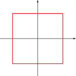1) A square is mathematically a set of points (for example, the four corner points are part of this set) and a symmetry of the square is a transformation that maps this set of points into itself.

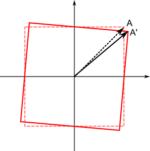Examples of symmetries of the square are certain (not all!) rotations about the origin. Certain rotations about the origin map the square into itself. This means, they map every point of the set to a point that lies again in the set, and the one says, the set is invariant under such a transformation.

This becomes obvious if we focus on the corner points of the square. Transforming the set by a clockwise rotation by, say 5°, maps these points into points outside th Einheitsquadrat-gedreht2 e original set that defines
the square. For instance, the corner point $A$ is mapped to the point $A’$, which is not found inside the set, that defined the square in the first place. Therefore a rotation by 5° is not a symmetry of the square. Of course, the rotated object is still a square, but not the same square (read: set of points). Nevertheless, a clockwise rotation by 90° is a symmetry of the square because the point $A$ is mapped to the point $B$, which lies again in the original set. Other examples of symmetry transformations of the square would be rotations by 180°, 270° and of course 0°.

Another perspective: Imagine you close your eyes for a moment, and then someone transforms the square in front of you. If you can’t tell after opening your eyes again if the other person changed anything at all, the transformation the person performed was a symmetry transformation.

The set of transformations that leave the square invariant is called a group. The transformation parameter, here the rotation angle, can’t take on arbitrary values and the group is called a discrete group.

2) Another example is the set of transformations that leave the unit circle invariant. Again, the unit circle is defined as a set of points and a symmetry transformation is a map, that maps this set into itself.

The unit circle is invariant under all rotations about the origin, not just a few. In other words: the transformation parameter (the rotation angle) can take on arbitrary values, and the group is said to be a continuous group.

Of course, mathematics isn’t exclusively about geometric shapes and one can find symmetries of different kinds of objects, too. For instance, considering vectors, one can look at the set of transformations that leave the length of any vector unchanged. (The object that is unchanged in this case is the metric, which is the mathematical object that defines length.) For this reason, the definition of symmetry I gave at the beginning was very general: Symmetry means invariance under a transformation. Luckily, there is one mathematical tool, called group theory, that lets us work with all kinds of symmetries. (As a side note: group theory was invented historically to investigate symmetries of equations).

To make the idea of a mathematical tool that lets us deal with symmetries precise, we need to distill the defining features of symmetries in a mathematical form:

- Leaving the object in question unchanged (“doing nothing”) is always a symmetry and therefore, every group needs to contain an identity element. In the examples above, the identity element is the rotation by 0°.

- Transforming some object and performing afterwards the inverse transformation must be equivalent to doing nothing. Therefore, there must be, to every element in the set, an inverse element. A transformation followed by its inverse transformation is, by definition of the inverse transformation, the same as the identity transformation. In the above examplesthis means that the inverse transformation to a rotation by 90° is a rotation by -90°. A rotation by 90° followed by a rotation by -90° is the same as a rotation by 0°.

- Performing a symmetry transformation followed by a second symmetry transformation is again a symmetry transformation. A rotation by 90° followed by a rotation by 180° is a rotation by 270°, which is a symmetry transformation, too. This property is called closure.

- The combination of transformations must be associative. A rotation by 90° followed by a rotation by 40°, followed by a rotation by 110° is the same as a rotation by 130° followed by a rotation by 110°, which is the same as a rotation by 90° followed by a rotation by 150°. In a symbolic form: $R(110°) R(40°) R(90°)= R(110°) \big(R(40°) R(90°)\big)= R(110°) R(130°)$ and $R(110°) R(40°) R(90°)=\big(R(110°) R(40°) \big) R(90°)= R(150°) R(90°)=$ This is called associativity. (This may not be confues with commutativity, because a the elements of a group, in general, do not commute. For example rotations around different axes: $R_x(30^\circ) R_z(40^\circ) \neq R_z(40^\circ) R_x(30^\circ) $)

- To be able to talk about the things above one needs a rule, to be precise: a binary operation, for the combination of group elements. In the above examples, the standard approach would be to use rotation matrices and the rule for combining the group elements (the corresponding rotation matrices) would be ordinary matrix multiplication. Nevertheless there are often different ways of describing the same thing. The rotations in the plane can be described by multiplication with unit complex numbers, too. Therefore, the rule for combining group elements would be complex number multiplication. Happily, group theory lets one study such, maybe confusing, diversity in a very systematic way. This branch of group theory is called representation theory, and we will have a look at it in another post.

We are now able to see that the abstract definition of a group simply states (obvious) properties of symmetry transformations:

A group is a set $G$, together with a binary operation $\circ$ defined on $G$ that satisfies the following axioms

Closure: For all $g_1, g_2 \in G$, $g_1 \circ g_2 \in G$
Identity: There exists an identity element $e \in G$ such that for all $g \in G$, $g \circ e = g = e \circ G$
Inverses: For each $g \in G$, there exists an inverse element $g^{-1} \in G$ such that $g \circ g^{-1}=e = g^{-1} \circ $ g.
Associativity: For all $g_1, g_2, g_3 \in G$, $g_1 \circ (g_2 \circ g_3) = (g_1 \circ g_2) \circ g_3$.

Why Group Theory?

Group theory is the branch of mathematics one uses to work with symmetries. A symmetry of an object is a transformation that leaves the object unchanged. The word object is chosen purposefully, because it is very vague. There is one branch of mathematics that deals with all kinds of symmetries, any kind of object can have.

The most familiar type of symmetries that come to one’s mind are symmetries of geometric shapes, so lets start with that.

Symmetries of Geometric Shapes

A square is defined mathematically as a set of points. A symmetry of the square is a transformation that maps this set of points into itself. This means concretely that by the transformation, no point is mapped to a point outside of the set that defines the square.

Obvious examples of such transformations are rotations, by $90^\circ$, $180^\circ$, $270^\circ$, and of course $0^\circ$.

A counter-example is a rotation by, say $5^\circ$. The upper-right corner point $A$ of the square is obviously mapped to a point $A’$ outside of the initial set. Of course, a square still looks like a square after a rotation by $5^\circ$, but, by definition, this is a different square, mathematically a different set of points. Hence, a rotation by $5^\circ$ is no symmetry of the square.

A characteristic property of the symmetries of the square is that the combination of two transformations that leave the square invariant, is again a symmetry. For example, combining a rotation by $90^\circ$ and $180^\circ$ is equivalent to a rotation by $270^\circ$, which is again a symmetry of the square. We will elaborate on this in the next post. In fact, the basic axioms of group theory can be derived from such an easy example.

Next, lets turn to something completely different.

Symmetries of Numbers?

Take a look at the fourth roots of unity, i.e., the (complex) numbers $z$ that give $1$ when raised to the fourth power:

\begin{equation} z^4 \stackrel{!}{=}1. \end{equation}

We can compute the solutions using the De Moivre Formula:

\begin{equation} z^n= (\cos(x)+i\sin(x))^n= \cos(nx)+i\sin(nx) \end{equation}

which follows when we write the complex number, using the Euler’s formula, as $\mathrm{e}^{ix}=\cos(x)+i\sin(x)$. The De Moivre Formula here yields,

\begin{equation} z^4= \cos(4x)+i\sin(4x) \stackrel{!}{=}1. \end{equation}

We know $\cos(2πk) + i \sin(2πk)=1$ for any integer k. The fourth roots of unity are

\begin{equation} z_k= \cos(2πk/4) + i \sin(2πk/4) \qquad \mathrm{ \ for} \qquad k = 0,1,2,3. \end{equation}

\begin{equation} \rightarrow z_0 = 1 \qquad , \qquad z_1 = i \qquad , \qquad z_2= -1 \qquad , \qquad z_3 = -i \qquad , \qquad \end{equation}

We can find a curious property of these numbers: The multiplication of two such solutions result again in a solution. Drawing the solutions in the complex plane gives us a geometric interpretation of this fact. The multiplication rotates any complex number by exactly the correct amount into another solution. The set of solutions is said to be closed under multiplication: By mere multiplication we can’t get any number that doesn’t lies in this set.

We have thus found a very similar structure in two completely different objects. On the one hand symmetries of the square, on the other hand the fourth roots of unity. Both sets contain exactly 4 objects and both share the property called closure: the combination of two objects in this set, lies again in the set. This indicates that there might be a map between the two sets, and indeed rotations in two-dimensions can be described by complex number multiplication. Exploring such intersections and structures in a systematic way is what group theory is all about.

Closure holds in general, for the n-th roots of unity, because, given two n-th roots $z,z’$, i.e. numbers for which $z^n=1$ and $z’^n=1$ holds, we have

\begin{equation} (z z’)^n = z^n z’^n = 1 \cdot 1 = 1 \quad \end{equation}

It’s no surprise that there exists a similar close relationship between the fifth-roots of unity and the symmetries of the pentagon.

We can search for higher order roots of unity and draw them in the complex plane. For example, the 100-th roots of units, i.e., the complex numbers satisfying $z^100 =1$, look like this:

These numbers are again closely related to the symmetries of a geometric object, that I don’t know the name of. Nevertheless, we can see where we are heading if we choose $n$ in $z^n=1$ to be larger and larger. Finally, we arrive at the unit circle,

The circle is quite different from the square and the pentagon, because the circle has infinitely many symmetries. Any rotation about the origin maps the circle into the circle. Such symmetries, called continuous symmetries, are the topic of a special branch of group theory, called Lie theory (after its inventor Sophus Lie).

Mathematics is a vast field. What started with integers and geometric shapes 2000 years ago, has become incredible diversified. Particular interesting things often happen at the intersection of branches of mathematics that don’t seem to have anything in common. Group theory is a framework that helps exploring such intersections.