Jakob Schwichtenberg

Demystifying the QCD Vacuum: Part 3 – The Untold Story

Although the subtle things that are often glossed over in the standard treatment of the QCD vacuum can be explained as discussed in part 2, there is another, more intuitive way to understand it.

Most importantly, this different perspective on the QCD vacuum shines a completely new light on the mysterious $\theta$ parameter.

To the expert, this perspective will be familiar. It sometimes appears in the literature and therefore the “untold” part in the headline is, of course, a bit exaggerated. However, it took me, as a student, a long long time to find it at all and most importantly a proper explanation that made sense to me.

The standard story of the QCD vacuum uses the temporal gauge. This is not a completely fixed gauge. Time-independent gauge transformations are still allowed. Only this residual gauge freedom makes the whole discussion in terms of large and small gauge transformations, etc. possible.

One may wonder what happens when we analyze the vacuum in a different gauge, where there is no residual gauge freedom. In other words: in a gauge that fixes the gauge freedom completely. Possibly choices are, for example, the axial and the Coulomb gauge.

The interpretation of the QCD vacuum is completely different in these gauges. Most importantly: there is no vacuum periodicity.

In the axial gauge, there is only one non-degenerate ground state. Then, of course, it is natural to wonder what we can learn about the $\theta$ parameter here. At a first glance, the result that there is a unique ground state implies that we have $\theta=0$. However, this is not the case and we will discuss this in a moment.

In the Coulomb gauge, there is only a non-degenerate ground state, too. However, the interpretation of the vacuum structure in this gauge is especially tricky. Most famously, one encounters the famous Gribov ambiguities. These appear because the condition that fixes the Coulomb gauge does not lead to unique gauge potentials everywhere in spacetime. Instead, there are regions where there are multiple gauge potential configurations that satisfy the condition. These configurations are called Gribov copies and the fact that we do not get a unique gauge potential configuration everywhere in spacetime is called Gribov ambiguity.

Now, how is this not a contradiction to the standard picture of the QCD vacuum? When there is only a unique non-degenerate ground state, there is no tunneling between degenerate vacua and therefore no $\theta$ parameter, right?

No! There is still tunneling and also a $\theta$ parameter. In the axial gauge, the tunneling starts from the unique ground state and ends at the same unique ground state. (In the Coulomb gauge the tunneling happens between the Gribov copies?!)

To understand this, we need an analogy.

A nice analogy to the QCD vacuum is given by the following Hamiltonian:

$$ H= – \frac{d^2 }{d x^2} + q(1-cos x) ,$$

where $-\infty \leq x \leq \infty$ and which describes a particle in a periodic potential $V(x) = q (1-cos x)$. Therefore, this situation is quite close to the standard picture of the QCD vacuum, with a periodic structure and infinitely many degenerate ground states.

Source: https://arxiv.org/abs/1505.03690

For this Hamiltonian, we have the Schrödinger equation

$$ – \frac{d^2 \psi}{d x^2} + q(1-cos x) \psi = E \psi . $$

(Among mathematicians this equation is known as the “Mathieu equation”. Sometimes it’s useful to know the name of an equation, if you want to dig deeper.)

However, exactly the same Hamiltonian describes a “quantum pendulum”. This interpretation only requires that we treat our variable as an angular variable: $x \to \phi$, with $0 \leq \phi \leq 2 \pi$ and thus

$$ – \frac{d^2 \psi}{d \phi^2} + q(1-cos \phi) \psi = E \psi . $$

Now, we identify the point $2 \pi$ with $0$ and all values of $\phi$ that are larger than $2 \pi$, with the corresponding points in the interval $0 \leq \phi \leq 2 \pi$. This implies immediately that $ \Psi(\psi + 2\pi) = \Psi(\psi) $. Therefore, the situation now looks like this:

and we no longer have infinitely many degenerate ground states, but only a unique ground state! Therefore, the situation here is exactly the same as for the QCD vacuum in a physical gauge.

Now, what about tunneling?

For a long pendulum, i.e. for large $q$, the ground state $\psi =0$ and excited states are approximately the same as for a harmonic oscillator. For large $q$, we can do a perturbative analysis in $q^{-1/2}$ and take the “anharmonicity” this way into account. However, the famously this perturbation series does not converge, because we miss something important in our analysis. Even for a pendulum with small energy, i.e. with only small perturbations around the ground state, the pendulum can “tunnel”. In this context, this means that the pendulum does a motion that it isn’t allowed to do, like rotate once around its suspension and end up again and the ground state. This is exactly what the instantons describe in a physical gauge like the axial gauge. There is no tunneling between degenerate ground states because there are no degenerate ground states. Instead, we have tunneling that starts at the unique ground state and ends again at the unique ground state. Still, this is tunneling, because there is a potential barrier that prohibits that a pendulum rotates once completely around its suspension. For a pendulum with low energy, or equally a long pendulum (large $q$), we can do the usual quantum mechanical perturbation analysis. This yields harmonic oscillator states plus small corrections from the anharmonicity. However, we must take into account that there are also quantum processes, like the tunneling once around the suspension of the pendulum.

Okay, fine. But what about $\theta$?

Well, now that we have understood that there can also be tunneling in the physical gauge picture of the QCD vacuum, which corresponds to the pendulum interpretation of the Hamiltonian in the example above, we can argue that there can be again a $\theta$ parameter. This is the phase that the pendulum picks up when it tunnels around its suspension. In a quantum theory, we can have $\Psi(\psi + 2\pi) = e^{-i \theta} \Psi(\psi) $ instead of $ \Psi(\psi + 2\pi) = \Psi(\psi) $.

When we interpret the Hamiltonian in the example above as the movement of a particle in a periodic potential, the parameter $\theta$ describes different states in the same system, completely analogous to the Bloch momenta in solid-state physics.

However, in the pendulum interpretation different $\theta$ describe different systems, i.e. different pendulums! Thus, in this second interpretation, it is much clearer why $\theta$ is a fixed parameter and not allowed to change.

To bring this point home, let’s consider an explicit example how a $\theta$ parameter can arise for the quantum pendulum.

The pendulum only picks up a phase $\theta$, when it moves in an Aharonov-Bohm potential. To make this explicit, let’s assume the pendulum carries electric charge $e$ and rotates around a solenoid with magnetic flux $\theta$. This magnetic flux is the source of a potential $ A$ in the plane of the rotating pendulum.

We get the Hamiltonian that describes this system by replacing the derivative with the covariant derivative:

$$ H= – \left(\frac{d }{d \phi} -ie A\right)^2+ q(1-cos \phi)  ,$$

and thus we have the Schrödinger equation

$$ – \left(\frac{d }{d \phi} -ie A\right)^2 \psi+ q(1-cos \phi) \psi= E \psi .$$

As before, we impose the condition $ \Psi(\psi + 2\pi) = \Psi(\psi) $. However, we can also introduce a new wave function $\varphi (\psi) $ that obeys the standard Schrödinger equation without the additional vector potential

$$ – \frac{d^2 \varphi}{d \phi^2} + q(1-cos \phi) \varphi = E \varphi ,$$

where

$$ \psi(\phi) = \text{exp} \left[ ie \int_0^\phi A d\phi \right] \varphi(\phi).$$

(Take note that the relation between the magnetic flux $\theta$ and the potential $A$ is $ \int_0^{2\pi} A d\phi = \theta $).

The information about the presence of the magnetic flux and hence of the vector potential $ A$ is now, when we use $\varphi(\phi)$ instead of $\Psi (\phi)$, encoded in the boundary condition:

$$ \varphi(\phi + 2\pi) = e^{-ie\theta} \varphi(\phi). $$

The energy of the ground state of the pendulum is directly proportional to the magnetic flux:

$$ E (\theta) \propto (1- \cos(\theta)) .$$

This show that in this model, the parameter $\theta$ defines different systems, namely quantum pendulums in the presence of different Aharonov-Bohm potentials.

In contrast, in the periodic potential picture, where $\theta$ is interpreted as analogon to the Bloch momentum, the parameter $\theta$ describes different states of the same system.

The reinterpretation of the QCD vacuum in a physical gauge with a unique non-degenerate vacuum, thus makes the appearance of $\theta$ much less obvious. This is why the standard presentation of the topic still makes use of the temporal gauge and the periodic vacuum picture.

The analysis of the QCD vacuum in the axial gauge is analogous to the interpretation of the Hamiltonian $$ H= – \frac{d^2 }{d \phi^2} + q(1-cos \phi) $$ as description of a quantum pendulum, i.e. substituting $x \to \phi$, with $0\leq \phi < 2 \pi$. (This interpretation also arises, when we work in the temporal gauge and declare that all gauge transformations (large and small) should not have any effect on the physics. The distinct degenerate vacua in the usual interpretation are connected by large gauge transformations. )

Without any further thought, one reaches immediately the conclusion that there is no $\theta$ parameter here. However, this is not correct, because a $\theta$ parameter can appear when there is an Aharonov-Bohm potential present.

When the quantum pendulum swings in such a potential, it picks up a phase when it rotates once around the thin solenoid that encloses the magnetic flux. The phase is directly proportional to the magnetic flux in the solenoid.

For the QCD vacuum, the same story goes as follows. In the axial gauge, naively there is no $\theta$ parameter because we do not have a periodic potential and hence no Bloch-momentum. However, nothing forbids that we add the term

$$ – \frac{g^2 \theta}{32\pi^2} Tr(G_{\mu\nu} \tilde{G}^{\mu\nu}),$$

where $\tilde{G}^{\mu\nu}$ is the dual field-strength-tensor: $\tilde{G}^{a,\mu \nu} = \frac{1}{2} \epsilon^{\mu \nu \rho \sigma} G^a_{ \rho \sigma}$, to the Lagrangian. This simply means that we allow for the possibility that there is an Aharonov-Bohm type potential and that it could make a difference when the pendulum rotates once around its suspension.

An obvious question is now, what the analogon to the solenoid is for the QCD vacuum. So far, I wasn’t able to find a satisfactory answer. The usual argument for the addition of $ – \frac{g^2 \theta}{32\pi^2} Tr(G_{\mu\nu} \tilde{G}^{\mu\nu})$ to the Lagrangian is that nothing forbids its existence.

So far, all experimental evidence point in the direction that there exists no “solenoid” for the QCD vacuum and therefore $\theta =0$. (The current experimental bound is $\theta < 10^{-10}$, Source).

From the analysis of the QCD vacuum in the axial gauge and by comparing it to the quantum pendulum, this does not look too surprising. However, we shouldn’t be too quick here and state $\theta =0$. Before we can say something like this, we need to understand first, what the “solenoid” could be for the QCD vacuum.

Understanding this requires that we enter a completely different world: the world of anomalies. This fascinating topic deserves its own post. Usually, it is claimed that the contribution to $\theta$ that comes from this sector of the theory is completely unrelated to the QCD $\theta$. However, we will see that anomalies and the QCD vacuum aren’t that unrelated: So far, we were only concerned with the gauge boson vacuum, while anomalies arise when we consider the fermion vacuum and its interaction with gauge bosons!

This will be discussed in part 4 of my series about the QCD vacuum.

References that describe this perspective of the QCD vacuum

  • “Topology in the Weinberg-Salam theory” by N. S. Manton
  • “The Interpretation of Pseudoparticles in Physical Gauges” by Claude W. Bernard, Erick J. Weinberg
  • Section 11.3 in Rubakov’s “Classical Theory of Gauge Field”
  • This perspective of the QCD vacuum in more abstract terms without the quantum pendulum analogy is described in “Introduction to the Yang-Mills Quantum Theory” by R. Jackiw in the around Eq. (42).

Demystifying the QCD Vacuum: Part 2 – The Subtleties No One Talks About

This is part two of my series about the QCD vacuum. You should only read this if you are confused about several things that are glossed over in the standard treatments. It turns out, that if you dig a bit deeper, these several such small things aren’t as obvious as most authors want you to believe. I already mentioned the problems with the two assumptions that are made in the standard texts without proper explanations. Here I will discuss the assumptions in more detail.

My main focus is answering the questions: Why there is so much emphasize on gauge transformations that become trivial at infinity $g(r, \phi , \theta) \to 1 $ for $r \to 1$ and why do the usual discussions make use of the temporal gauge? I already discussed in the first post, why these assumptions are absolutely crucial. Without them, there is no way to arrive at the standard interpretation of the QCD vacuum.

These two things only make sense, when you know something about constrained Hamiltonian quantization and Gauss’ law.

Only if you have some basic understanding of these two notions, you can truly understand the ideas of the discoverers of the non-trivial structure of the QCD vacuum.

My plan is to write more about both, constrained Hamiltonian quantization and Gauss’ law, in the future, but just to demonstrate that both are an interesting topic on their own, regardless of the QCD vacuum, here are two quotes:

“The constrained Hamiltonian formalism is recommended as a means for getting a grip on the concepts of gauge and gauge transformation. This formalism makes it clear how the gauge concept is relevant to understanding Newtonian and classical relativistic theories as well as the theories of elementary particle physics; it provides an explication of the vague notions of “local” and “global” gauge transformations; it explains how and why a fibre bundle structure emerges for theories which do not wear their bundle structure on their sleeves; it illuminates the connections of the gauge concept to issues of determinism and what counts as a genuine “observable”; and it calls attention to problems which arise in attempting to quantize gauge theories. “ Gauge Matters by John Earman


“The main output of this analysis is therefore the suggestion that Gauss law is the basic and primary feature which characterized elementary particle interactions, rather than gauge invariance, a concept which is more difficult to grasp on physical grounds since it can be given a meaning only by introducing unobservable quantities. Gauge Invariance can therefore be regarded as a technical tool for constructing Lagrangian functions or equations of motion which guarantee the validity of Gauss’ law. This may be the right track to get an insight into the structure of GQFT and possibly understand why nature seems to choose gauge theories for elementary particle interactions.”
Gauss’ Law in Local Quantum Field Theory by F. Strocchi

This post should be about how these concepts help to understand the standard discussion of the QCD vacuum and therefore I will keep discussions that would lead us too far apart to a minimum.

So, without further ado, let’s get started.

How do we get a Quantum Theory?

In modern physics, when we write down a model to describe a given system, we start with a Lagrangian. This is clever because the Lagrangian framework is ideal to make use of symmetry considerations. If the Lagrangian (or better, the action) is invariant under some transformation, the equations of motion, have this symmetry, too.

In contrast, for example, the Hamiltonian, is not even invariant under Lorentz transformations as it represents the energy and is thus only one component of a Lorentz vector, the four momentum. Therefore, it is much harder to “guess” the correct Hamiltonian that describes the system in question.

However, when we want to describe a quantum system, a Lagrangian is not enough. Although we get from the Lagrangian the equations of motion via the Euler-Lagrange equations, these are not enough to describe the quantum behavior of the system. The equations of motions are, on their own, purely classical and there is nothing quantum about them.

Thus, we need additional equations that describe the quantum behavior and we get them through the process called “quantization”.

There are different ways to quantize a given classical system, but one popular and famous possibility is the constrained Hamiltonian quantization procedure. (A now-popular alternative is the path-integral formalism. However, the canonical procedure described below makes many points more transparent).

This is a reliable way to quantum physics and the main points are well known to most students. We derive from the Lagrangian the canonical momenta and then quantize the system by replacing the classical Poisson bracket with the quantum commutator (or anticommutator)

$$ \{ \cdot , \cdot \} \to \frac{1}{i\hbar} [\cdot , \cdot ]. $$

However, there are several subtle points that need to be taken care of when we try to use this procedure.

While you may not care about such “details”, it is absolutely crucial to understand this procedure, if you want to understand the standard picture of the QCD vacuum that is repeated in almost all textbooks and reviews. In addition, hopefully, the quote above has sparked some interest that there is something deep that we can learn here.

For our purpose here, however, it is only important to know that the guys who came up with the standard interpretation of the QCD vacuum cared about this procedure a lot.

To (canonically) quantize, we must compute the generalized momenta $p_i$ for the given Lagrangian and then impose the famous commutation relations $[q_i,p_j]= i \delta_{ij}$.

We also need these generalized momenta to get the Hamiltonian that corresponds to the given Lagrangian. We need the Hamiltonian in the canonical formalism, for example, to calculate the time-evolution of quantum fields.

The mathematical procedure to get the Hamiltonian from a given Lagrangian and thus to get the generalized momenta is called Legendre transform.

However, this procedure is not as straight-forward as one would naively assume. The Lagrangian is a function of $q_i$ and $\dot{q}_i$, whereas the Hamiltonian is a function of $q_i$ and the generalized momenta and $p_i$. The Legendre transform is the process to calculate from the generalized velocities $\dot{q}_i$ the corresponding generalized momenta $p_i$:

$$ p_i \equiv \frac{\partial L }{\partial \dot{q}_i} .$$

In principle, we can invert this definition and get the generalized velocities as a function of $q$ and $p$: $ \dot{q}_i = \dot{q}_i (q_i,p_i)$.

However, for some systems, these relations are not invertible. Instead, not all momenta are independent and we get a family of constraints that the momenta must satisfy

$$ f_a(q,p) =0 \quad a=1,…,N $$

These constraints are the reason why this formalism is called constrained Hamiltonian quantization.

Glossing over some details (the process of finding all independent constraints and the definition of “first-class” constraints, which are those constraints whose mutual Poisson bracket vanishes), the crucial thing is now that the constraints generate gauge transformations!

The understand this, we note that the correct total Hamiltonian is given by the “naive” Hamiltonian $H_T$ plus a linear combination of all (first class) constraints with arbitrary coefficients

$$ H_T = p_i \dot{q}_i – L + \sum_{a=1}^N \lambda_a(t) f_a.$$

(The implementation of constraints in this way is known as the method of “Lagrange multiplies”)

The Hamiltonian describes the time evolution of the system in question. The additional terms here mean that there is an ambiguity in the time evolution and this ambiguity is exactly our gauge freedom!

The origin of these complications, can be traced back to the equations of motions in the Lagrangian framework

$$ \frac{\partial^2 L}{\partial \dot{q}_i \partial \dot{q}_j } \ddot{q}_j= – \frac{\partial^2 L}{\partial \dot{q}_i \partial q_j } \dot{q}_j + \frac{partial L}{\partial q} . $$

The accelerations can only be determined in terms of the positions and velocities if the Jacobian matrix of the transformation $(q_i, \dot{q}_i) \to (p_i, p_i)$:

$$\frac{\partial p^i}{\partial \dot{q}_j} = \frac{\partial^2 L}{\partial \dot{q}_i \partial \dot{q}_j } \ddot{q}_j$$

is non-singular. Only then, the transformation is unique and the canonical quantization procedure works without subtleties.

This can be seen, by analyzing the equation $\det\left( \frac{\partial^2 L}{\partial \dot{q}_i \partial \dot{q}_j } \ddot{q}_j \right) =0 $. This equation implies that some of the momenta aren’t independent variables.

This means, we have constraints when the determinant of the Jacobian matrix is zero and therefore the time evolution is not uniquely determined in terms of the initial conditions.
(For more on this, see, for example, this paper).

This is a very special perspective on gauge freedom that isn’t very familiar to students nowadays. However, it is absolutely crucial to understand what the discoverers of the non-trivial structure of the QCD vacuum had in mind.

A concrete example may be helpful.

Constrained Quantization of Electrodynamics

The Lagrangian of electrodynamics is $L = – \frac{1}{4} \int d^3xF_{mu\nu} F^{\mu\nu}$ and contains some gauge freedom. This becomes especially transparent when we try to quantize electrodynamics by following the procedure described above.

The path from this Lagrangian to the correct description in the Hamiltonian framework is quite subtle because we have here an explicit example, of the situation described above.

When we calculate the generalized momenta to $A_\mu$:

$$ \pi^\mu = \frac{\partial L}{\partial (\partial_0 A_\mu)}= F^{\mu 0}, $$

we get $\pi^0 =0$ and $\pi = E^i$, where $E$ is the usual electric field. Thus, we notice here the constraint: $\pi^0 =0$.

Following, the procedure described above, we have the following total Hamiltonian
$$ H_T = \int d^3x \left( \pi^\mu \partial_0 A_\mu – \mathcal{L} \right) + \int d^3x \lambda_1(x) \pi_0(x)$$
$$ \int d^3 x \left( \frac{1}{2} (\vec{E}^2 +\vec{B}^2) + A_0 \Delta \cdot \vec E \right) + \int d^3x \lambda_1(x) \pi_0(x) $$

(In this calculation, one uses $\partial_0 \vec A = \Delta A_0 -\pi = \Delta A_0 – \vec E$ and integrates the second term by parts.)

We recognize the first term here $\propto \frac{1}{2} (\vec{E}^2 +\vec{B}^2)$ as the well known electromagnetic field energy density. The last term is the implementation of the constraint $\pi_0(x) =0$ via a Lagrange multiplier $\lambda_1(x)$. What about the second term?

To understand this second term, let’s take a step back and go back to the Lagrangian.

One of the equations of motions that we get via the Euler-Lagrange equations from the Lagrangian $L = – \frac{1}{4} \int d^3xF_{mu\nu} F^{\mu\nu}$, is Gauss’ law:

$$ \Delta \cdot \vec E = 0. $$

(Gauss’ law is, of course, one of the famous Maxwell equations. In words, Gauss law simply states that the flux of the electric field from a volume is proportional to the charge inside. In electrodynamics without sources, which is what we consider here with our Lagrangian, this flux is therefore zero.)

However, take note that it is a very special kind of “equation of motion”. It contains no time-derivatives and therefore does not describe any time-evolution. Hence it is not really an equation of motion!

If we now have again a look at the Hamiltonian that we derived above, we can see that the second term has exactly the same structure as the third term. The equation $ \Delta \cdot \vec E = 0$ is a constraint, exactly as $\pi_0(x) $. The Lagrange multiplier for this term is simply $A_0(x)$.

Our two (first class) constraints are $\pi_0 =0$ and $\Delta \vec{\pi } = \Delta \vec{E}=0$. In the Hamiltonian framework, they show up as constraints that we implement by making use of Lagrange multipliers.

Now that we know that $A_0(x)$ is not really a dynamical variable, it seems reasonable to simplify our calculations by choosing the temporal gauge $A_0(x)=0$. (It can already be seen from the Lagrangian that $A_0(x)$ is not a dynamical variable because there is no time derivative of $A_0(x)$ in the Lagrangian.)

However, $A_0(x)=0$ is not a complete gauge fixing. We still have the freedom to perform time-independent gauge transformations. This remaining gauge freedom can be fixed, for example, by the demand $\Delta \cdot \vec A =0$.

When we recall the remark from above, that the constraints generate gauge transformations, we can understand the residual gauge freedom after fixing $A_0(x)=0$ from another perspective:

The choice $A_0(x)=0$ uses up the gauge freedom generated by $\pi_0 =0$ (called the momentum constraint). However, we still have the gauge freedom generated by Gauss’ law $\Delta \vec{E}=0$.

This can be seen, for example, by going back to the Lagrangian invoking Noether’s theorem for time-independent gauge transformations.

The conserved “charge” that follows from invariance under time-independent gauge transformations:

$$ Q_\phi = \int dr \pi_a \cdot \delta A_a = \frac{1}{g} \int_{-\infty}^\infty dr \vec {E}_a (\Delta \phi (r))_a $$

where $\phi(x)$ is the “gauge function”. This looks almost like Gauss’ law, but not exactly. Gauss law involves $\Delta \vec{E}$, whereas here $\Delta $ acts on the gauge function $\phi(x)$. However, we can rewrite this Noether charge such that it contains $\Delta \vec{E}$ by integrating by parts.

When we integrate by parts, we get a boundary term $( \frac{1}{g} \vec {E}_a \phi (r)_a \big |_{-\infty}^\infty $. We can only neglect this boundary term, when $\phi (-\infty) = \phi (\infty) =0$.

This is a subtle point that is often glossed over (see, for example, Eq. 3.22 in Topological investigations of quantized gauge theories by R. Jackiw, where this “glossing over” is especially transparent). The subtle and small observation that $\theta (-\infty) = \theta (\infty) =0$ is a requirement for Gauss’ law to be a generator of gauge transformations will become incredibly important in a moment.

Forgetting this “detail” for a moment, we can conclude $ E_a\cdot \Delta$ is conserved. This can also be verified, by computing the explicit commutator with the Hamiltonian. Noether charges always generate the corresponding symmetry transformations and in this sense, $ E_a\cdot \Delta$ generates time-independent gauge transformations. The Noether “charge” for time-independent gauge transformations is $\propto \Delta E$ and hence this is the generator of such gauge transformations.

(A second possibility to see that Gauss’ law generates gauge transformations is to consider the explicit commutator of $G_a = – \frac{1}{g} (\Delta E)$ and the electrical potential $A_b$ and the electrical field $E_a$. Moreover, we can compute that $\frac{i}{\hbar} [H,G_a]=0$ and therefore $G_a$ is indeed conserved. )

Gauss’ Law in a Quantum Theory

Now, let’s remember that we want to talk about a quantum theory. It is somewhat a problem what to make of Gauss’ law in a quantum theory.

On the one hand, we can invoke the equal-time commutation relations and compute

$$ [G_a (x_1),A_1(x_2)]_{t=0} = i \partial_{x_1} \delta (x_1-x_2) \neq 0 .$$

On the other hand, we have the explicit statement of Gauss’ law, that $ G_a = \Delta \cdot \vec E_a = 0$

The crucial idea to resolve this “paradox” is to take the idea that Gauss’ law is a constraint seriously. Hence, the operator $G_a$ is not zero, but when it acts on states we get zero.

In the classical theory, Gauss’ law is a restriction on the initial data. In the quantum theory, we now say that Gauss’ law defines physical states, via the equation $G |\Psi\rangle_{phys}=0$. Non-physical states can, by definition, do whatever they want and there is no need that they respect Gauss’ law. (This is the crucial idea behind the Gupta-Bleuler formalism).

Okay, this was a long convoluted story. What’s the message to take away here?

The Crucial Points to Take Away

The crucial point is that Gauss’ law only forces gauge equivalence under gauge transformations which are generated by $G_a$ and become trivial at spatial infinity.

Certainly, there are other possibly gauge transformations, but Gauss’ law has nothing to say about them.

Quantization is a science on its own and this post is not about quantization. However, I hope the few paragraphs above, make clear that when you come from the constrained Hamiltonian quantization perspective a few things are quite natural:

– $A_0(x) =0$ is an obvious choice to simplify further calculations.
– The residual gauge freedom after fixing $A_0(x) =0$ is generated by Gauss’ law. This gauge freedom includes only a very particular subset of gauge transformations. In the discussion above, we have seen that Gauss’ law only generates gauge transformations via $\text{exp}\left(\frac{1}{g} \int d^3 x \phi(\vec x)_a G_a\right)$ that include a gauge function that vanishes at infinity $\phi (-\infty) = \phi (\infty) =0$. When you come from the perspective of constrained Hamiltonian quantization, it makes sense to treat those gauge transformations that involve a gauge function that does become zero at spatial infinity as special. All other gauge transformations are not forced by Gauss law to leave physical states invariant.

Why Only Trivial Gauge Transformations?

Take note that we still haven’t fully elucidated that assumptions that were used in the first post to explain the standard story of the QCD vacuum.

So far, we have only seen why the gauge transformations with a gauge function that satisfies $\phi (-\infty) = \phi (\infty) =0$ is special because it is forced by Gauss’ law to be a symmetry of physical states.

We still have to talk about, why we restricted ourselves in the first post those gauge transformations that involve a gauge function that becomes a multiple of $2 \pi$ at spatial infinity, instead of all gauge transformations.

In other words, why was it sufficient to restrict ourselves to gauge transformations that become trivial at infinity $g(x) \to 1 $ for $|x| \to \infty$?

If you look through the literature, you will find many reasons. However, if you find many arguments, this is usually a red flag that things aren’t as bulletproof as people would like them to be.

I’m not the only one who feels this way. For example, Itzykson and Zuber write in their famous QFT book:

“there is actually no very convincing argument to justify this restriction”.

In addition, while Roman Jackiw (one of the founding fathers of the standard picture of the QCD vacuum) claimed in the original paper that this restriction $g(x) \to 1 $ for $|x| \to \infty$ simply follows because “we study effects which are local in space” (1976), he later became more careful. In his “Introduction to Yang-Mills theory” (1980) he wrote

We shall make a very important hypothesis concerning the physically admissible finite transformations. While some plausible arguments can be given in support of this hypothesis (see below) in the end we must recognize it as an assumption, without which the subsequent development cannot be made. We shall assume that the allowed gauge transformation matrices U tend to a definite limit as r passes to infinity

$$ lim_{r\to\infty} U(r)= U_\infty$$

Here $ U_\infty$ is a global (position-independent) gauge transformation matrix. With this hypothesis, we are excluding gauge transformations which do not have a well-defined or unique limit at $r \to \infty$.”

He then lists three arguments why this restriction is plausible. This is good style, but unfortunately, most other presentations of the QCD vacuum gloss over this important point and act like the restriction is obvious for some reason.

In fact, I have collected an even longer list with around 10 arguments that are put forward in textbooks and papers to justify the restriction $g(x) \to 1 $ for $|x| \to \infty$. Some are better than others and I think one is really strong, but ultimately one needs to admit that this restriction

“has always been recognized as weak but it had seemed necessary.” (Source)

Unfortunately, this recognition has not been loud and clear enough. Many students I have talked to think that this restriction has something do with the fact that we investigate “finite energy” solutions of the Yang-Mills equations. This, however, can not be correct, because the energy shouldn’t care about gauge transformations at all. Hence, there can be no reason that follows from some energy argument for the restriction to a subset of gauge transformations.

Another popular argument is that we need some boundary conditions and that our particular choice shouldn’t matter because we do not care about what happens at infinity. (See for example page 166 in “Quarks, leptons and gauge fields” by Huang, where he writes “It is a common article of faith to assume that boundary conditions at large distance have no effect on local phenomena”.). This argument is exactly what Jackiw proposed in his first paper I quoted above. However, this argument is hardly satisfactory. Our choice of boundary conditions shouldn’t make any difference. However, when we do not restrict ourselves to the subset that satisfies $g(x) \to 1 $ for $|x| \to \infty$, there is no homotopy discussion possible and the usual periodic vacuum picture does not emerge. Hence the boundary condition seems to make a big difference. Another way to see that this argument is problematic is to consider different definite boundary conditions. If they do not matter, so why not? For example, instead of $g(x) \to 1 $ for $|x| \to \infty$, which leads to a compactification of space to the sphere $\mathbb{R}^3 \to S^3$, we could consider a large box and impose periodic boundary conditions. Then space does not become a sphere, but a torus and the homotopy classification is completely different.

My favorite point of view is to ignore all these nasty things, by analyzing the QCD vacuum from a completely different perspective. I will describe this alternative description in the next post in this series.

But for now, how can we make sense of the restriction $g(x) \to 1 $ for $|x| \to \infty$?

We already know that the gauge transformations that involves a gauge function that becomes zero at infinity are special, because these are generated by Gauss’ law and hence are true symmetries of the physical states.

With this in mind, probably the best argument is that tunneling does only happens from a vacuum with winding number zero (i.e. one that is “Gauss’ law gauge equivalent” to $A_\mu =0$), to a vacuum state with integer winding number (i.e. one that we get from $A_\mu =0$ with a gauge transformation that satisfies $g(x) \to 1 $ for $|x| \to \infty$). If we can show this, it seems reasonable that we neglect other ground states are not reachable by tunneling processes.

To show this, imagine spacetime as a cylinder. Each slice of the cylinder is the complete space $\mathbb{R}^3$ at a given time $t$. The lower cap of the cylinder is space at $t = – \infty$ and the upper cap space at $t = \infty$. Now, we start at $t= -\infty$ with our quantum field in a vacuum configuration with winding number zero. We have the gauge freedom to choose $A_\mu (\vec x , -\infty) =0$. (However, take note that all other pure gauge configurations, that are generated by a Gauss’ law gauge transformation are equally valid. The gauge transformations generated by Gauss’ law are those that have a gauge function in the exponent that satisfies $f(x) \to 0$ for $|x| \to \infty$. All configurations that we get from $A_\mu(\vec x , -\infty) =0$ with such a gauge transformations are also winding number zero configurations, because they are gauge equivalent to $A_\mu(\vec x , -\infty) =0$.) Each pure gauge configuration of $A_\mu$, which means $A_\mu = U^\dagger (\vec x, t)\partial U(\vec x, t) $, is a vacuum configuration. $A_\mu (\vec x , -\infty) =0$ means $U(\vec x, -\infty) =\text{const}. $

This is the naive vacuum configuration and we want to investigate what non-trivial configurations of our quantum field are possible. We are especially interested in what the final configurations at $t = \infty$ can be.

Now, remember that we work in the temporal gauge. As already mentioned above, this choice of gauge does not fix the gauge freedom completely, but instead all time-independent gauge transformations are still permitted.

In addition, we are interested in finite energy processes. This requirement means that at spatial infinity our field energy must vanish, which means that our quantum field must be in a pure gauge configuration at spatial infinity. (This is discussed in more detail in the first post).

We now put these three puzzle pieces together:

At $t = – \infty$, we have $A_\mu(\vec x , -\infty) =0$ and therefore $U(\vec x, -\infty) =\text{const}. $ At the boundary, $A_\mu$ must stay pure gauge all the way from $t= – \infty$ to $t=\infty$: $A_\mu(\infty, t) = U^\dagger (\infty, t)\partial U(\infty, t) $.

The crucial thing is now that at $t = -\infty$, we started with a configuration that corresponds to $U(\vec x, -\infty) =\text{const}$. Thus at this time, we also have at spatial infinity $U(\infty, -\infty) =\text{const}$. In the temporal gauge, only time-independent gauge transformations are permitted. Therefore, $U(\infty, -\infty) =\text{const} = U(\infty, t) = U(\infty)$ is fixed and does not change as we time moves on!

Therefore, we also have at the upper cap of the cylinder, i.e. at $t=\infty$ are pure gauge configuration (because we consider a vacuum state to vacuum state transition) $A_\mu(\infty, \infty) = U^\dagger (\infty, \infty)\partial U(\infty, \infty) $ with $U(\infty, -\infty) =\text{const}$.

Hence, when we start with a vacuum configuration, which means a gauge transformation of $A_\mu =0$ with $U(\vec x, -\infty) =\text{const}$, our field can only transform into configurations that are gauge transformations of $A_\mu =0$ with $U(\vec x, \infty) =\text{const}$.

You may now wonder why the anything non-trivial is possible at all. The answer is that the restriction that $A_\mu$ must be pure gauge only holds:

– At the lower cap, i.e. for $A_\mu(\vec x , -\infty)$, because we start with a vacuum configuration.
– At the curved surface boundary of the cylinder, i.e. for $A_\mu(\infty, t)$, because we only consider finite energy process, which requires that the field energy vanishes at spatial infinity and thus that $A_\mu$ is pure gauge there.
– At the upper cap $A_\mu(\vec x , \infty)$, because we investigate vacuum to vacuum transitions.

Thus, in between, there is a lot of non-trivial stuff that can happen. Especially, on the way from the pure gauge at $t=-\infty$ to pure gauge $\infty$ it can be in non-pure-gauge configurations somewhere in space at some point in time. In other words, it is possible, within our restrictions that the field is, on the way from $t=-\infty$ to $t=\infty$, in a configuration that corresponds to non-zero field energy. These non-zero field energy configurations are exactly the potential barrier that we talked about in the first post. In this sense, we are dealing here with tunneling phenomena. We start with a vacuum state, i.e. zero field energy. Nevertheless, the field manages to get into configurations that “normally” would require energy to get into. However, because we are dealing with a quantum theory, it is possible that the field tunnels through these, classically forbidden configurations.

Only because this is, in principle possible, does not mean that it actually happens. However, there are solutions of the Yang-Mills equations that exactly describe such processes: the famous instanton solutions. Thus it seems reasonable that such tunneling indeed happens. (It is really cool to see how an instanton solution describes the process of how a vacuum configuration transforms into a different vacuum configuration. Different here means with a different winding number. However, there are already good descriptions in the literature and I’m currently not motivated to write down all the required formulas. An especially nice and explicit description can be found on page 168 (section 8.6.2 “Instantons as Tunneling Solutions”) in “Quarks, Leptons & Gauge Fields by Kerson Huang).

The crucial message of the description above is that we necessarily get a final field configuration that corresponds to a pure gauge configuration with $U(\vec x, \infty) =\text{const}$. The constant is necessarily the same constant that we started with at $t=-\infty$. Therefore, transitions only happen between pure gauge configurations that are generated by gauge transformations which have the same trivial limit at spatial infinity. (Trivial means that there is no dependence on angles, but instead the gauge transformation becomes the same constant no matter from which direction we approach $|x| = \infty$. )

Now, let’s connect this discussion with our previous discussion of Gauss’ law:

Recall that above we argued that the gauge transformations generated by Gauss’ law are somewhat special because we use Gauss’ law to identify physical states in a quantum theory. These gauge transformations are exactly those with a gauge function $f(x)$ in the exponent that becomes zero at spatial infinity: $U(x) = e^{if(x) \hat r \cdot \vec G}$ with $f(\infty) =0$. The naive vacuum configuration is $A_\mu=0$. All configurations that we get by transforming this configuration with a gauge transformation that is generated by Gauss’ law are completely equivalent to $A_\mu =0$, because that’s how we use Gauss’ law in a quantum theory. Therefore, starting from the naive vacuum configuration, or one that is physically equivalent, we have $U(\infty , – \infty) = 1$. Therefore, with the arguments from above, we can only end up in a configuration with $U(\infty, \infty)=1$, too!

In this sense, it is sufficient to restrict ourselves to gauge transformations that satisfy $U(x) \to 1$ for $|x| \to \infty$. This is the moral of this long story.

In my next post about the QCD vacuum, I will present another way to look at it. With this different interpretation, we can avoid all the confusing details

Demystifying the QCD Vacuum – Part 1 – The Standard Story

After being confused for several weeks about various aspects of the QCD vacuum, I now finally feel confident to write down what I understand.

The topic itself isn’t complicated. However, a big obstacle is that there are too many contradictory “explanations” out there. In addition, many steps that are far from obvious are usually treated in like two lines. I’m not going to flame against such confusing attempts to explain the QCD vacuum. Instead, I want to tell a (hopefully) consistent story that illuminates many of the otherwise highly confusing aspects.

The QCD vacuum is currently (again) a big thing. It was discussed extensively in the 80s and it is now again popular because there are lots of people working on axion physics. The axion mechanism is an attempt to explain what we know so far experimentally about the QCD vacuum. A careful analysis of the structure of the QCD vacuum implies that QCD, generally, violates CP symmetry. So far, no such violation was measured. This is a problem and the axion mechanism is one possibility to explain why this is the case.

However, before thinking about possible solutions, it makes sense to spend some time to understand the problem.

Usually, when we think about the vacuum, we don’t think that there is a lot to talk about. Instead, we have something quite boring in mind. Empty space. Quantum fields doing nothing, because they are, by definition, not excited.

However, it turns out that this naive picture is completely wrong. Especially the vacuum state of the quantum theory of strong interactions (QCD) has an incredibly rich structure and there are lots of things that are happening.

In fact, there is so much going on, that the vacuum isn’t fully understood yet. The main reason is, of course, that, so far, we always have to use approximations in quantum field theory. Usually, we use perturbation theory as the approximation method of choice, but it turns out that this is not the correct tool to describe the vacuum state of QCD.

The reason for this is that there are (infinitely) many states with the minimal amount of energy, ground states, and the QCD fields can change from one ground state into another. When we study these multitudes of ground states in detail, we find that they do not lie “next to each other” (not meant in a spatial sense) but instead there are potential barriers between them. The definition of a ground state is that the fields which are in this configuration, have the minimal amount of energy and thus certainly not enough to jump across the potential barriers. Therefore, the change from one ground state into another is not a trivial process. Instead, the fields must tunnel through these potential barriers. Tunneling is a well-known process is quantum mechanics. However, it can not be described in perturbation theory. In perturbation theory, we consider small perturbations of our fields around one ground state. Thus, we never notice any effects of the other ground states that exist behind the potential barriers. We will see below how this picture of infinitely many ground states with potential barriers between them emerges in practice.

The correct tool to describe tunneling processes in quantum field theory is to use a semiclassical approximation. At a first glance, this certainly seems contradictory. There is no tunneling in a classical theory, so why should a semiclassical approximation help to describe tunneling processes in quantum field theory? The trick that is used to make the semiclassical approximation work is to substitute $t\to i \tau$, i.e. to make the time imaginary. At first, this looks completely crazy. However, there are good reasons to do this, because it is this trick that allows us to use a semiclassical approximation to describe tunneling processes. Possibly the easiest way to see why this makes sense is to recall the standard quantum mechanical problem of an electron facing a potential barrier. Before the potential barrier, we have an ordinary oscillating wave function $e^{i\omega t}$. But inside the potential barrier, we find a solution proportional to $e^{-\omega t}$. Physically, this means that the probability to find the electron inside the potential barrier decreases exponentially. By comparing the tunneling wave function with the ordinary wavefunction, we can see that the difference is precisely described by the substitution: $t\to i \tau$. In addition, we will see below that the effect of $t\to i \tau$ is basically to flip the potential upside down. Therefore, the potential barrier becomes a valley and there is a classical path across this valley. The technical term for such a tunneling process is instanton.

If this didn’t convince you, here is a different perspective: In the path integral approach to quantum mechanics, we need to sum the action for all possible paths a particle can travel between two fixed points. The same is true in quantum field theory, but there we must sum over all possible field configurations between two fixed field configurations. Usually, we cannot compute this sum exactly and must approximate it instead. One idea to approximate the sum is to find the dominant contributions. The dominant contributions to the sum come from the extremal points of the action and these extremal points correspond exactly to the classical paths. For our tunneling processes, the key observation is that there are, of course, no classical paths that describe the tunneling. Thus, without a clever idea, we don’t know how to approximate the sum. The clever idea is, as already mentioned above, to substitute $t\to i \tau$. After this substitution, we can identify the dominant contributions to the path integral sum, because now there are classical paths. At the end of our calculation, after we’ve identified the dominant contributions, we can change back again to real-time $ i \tau \to t$. This is another way to see that a semiclassical approximation can make sense in a quantum field theory.

Now, after this colloquial summary, we need to fill in the gaps and show how all this actually works in practice. We start by discussing how the QCD vacuum picture with infinitely many ground states, separated by potential barriers, comes about. Afterward, we discuss how there can be tunneling between these ground states and then we write down the actual ground state of the theory. This real ground state is a superposition of the infinite number of ground states. The final picture of the QCD vacuum state will be completely analogous to the wave function of an electron in a periodic potential. In nature, such a situation is realized, for example, in a semiconductor. The electron does not sit at one of the many minimums, but is instead in a state of superposition, because it can tunnel from one minimum of the potential to another. The correct wave function for the electron in this situation is known as a Bloch wave. We find energy bands that are separated by gaps. The bands are characterized by a parameter $\theta$, which corresponds to the phase that the electron picks up when it tunnels from one minimum to another. Analogously, the real QCD ground state will be written as a Bloch wave and is equally characterized by a phase $\theta$. This phase is a new fundamental constant of nature and can be measured in experiments. However, so far, no experiment was able to measure $\theta$ for the QCD vacuum and we only know that it is incredibly small. In theory, the measurement is possible, because $\theta$ tells us to what extent strong interactions respect CP symmetry. The surprising smallness of $\theta$ is known as the strong CP problem. QCD alone says nothing about the value of $\theta$ and therefore it could be any number.

The QCD Vacuum Structure

The vacuum of a theory is defined as the state with the minimal amount of energy. In a non-abelian gauge theory, this minimal amount of energy can be defined to be zero and corresponds, for example, to the gauge potential configuration

$$ G_\mu = 0 . $$

However, this is not the only potential configuration with zero energy. Every gauge transformation of $0$ is also a state with minimal energy. The gauge potential transforms under gauge transformations $U$ as:

\begin{equation}
G_{\mu} \to U G_{\mu} U^\dagger -\frac{i}{g}U\partial_{\mu}U^{\dagger} .
\end{equation}

Putting $G_\mu = 0$ into this formula yields all configurations of the gauge potential with zero energy, i.e. all vacuum configurations:

\begin{equation}
G_{\mu}^{\left( pg\right) }=\frac{-i}{g}U\partial_{\mu}U^{\dagger}
\label{pureg}%
\end{equation}

Such configurations are called pure gauge.

This observation means that we have infinitely many possible field configurations with the minimal amount of energy. Each of these is a “classical” vacuum state of the theory. This may not seem very interesting because all these states are connected by a gauge transformation. Thus aren’t all these “classical” vacua equivalent? Isn’t there just one vacuum state that we can write in many complicated ways by using gauge transformations?

Well… to understand if things are really that simple, we need to talk about gauge transformations. Each “classical” vacuum of the theory corresponds to a specific gauge transformation $U$ via the formula

\begin{equation}
G_{\mu}^{\left( pg\right) }=\frac{-i}{g}U\partial_{\mu}U^{\dagger} .
\end{equation}

Now, the standard way to investigate the situation further is to mention the following two things as casually as possible

1.) We work in the temporal gauge $A_0 = 0$.
2.) We assume that it is sufficient to only consider those gauge transformations that become trivial at infinity $U(x) \to 1$ for $|x| \to \infty $.

Most textbooks and reviews offer at most one sentence to explain why we do these things. In fact, most authors act like assumptions are trivial and obvious or not important at all. As soon as these “nasty” technicalities are out of the way, we can start discussing the beautiful picture of the QCD vacuum that emerges under these assumptions. However, things aren’t really that simple. We will discuss the two assumptions in my second post about the QCD vacuum. Here I just note that they are not obvious choices and you need a very special perspective if you want to understand these choices.

For now, we simply summarize what we can say about our gauge transformations under these assumptions.

So, now back to the vacuum. We wanted to talk about gauge transformations, to understand if really all “classical” vacua are trivially equivalent.

We will see in a moment that the subset of all gauge transformations that fulfill the extra condition $U(x) \to 1$ for $|x| \to \infty $, fall into distinct subsets that can’t be smoothly transformed into each other. The interpretation of this observation is that these distinct subsets correspond via the formula $G_{\mu}^{\left( pg\right) }=\frac{-i}{g}U\partial_{\mu}U^{\dagger}$ to distinct vacua. In addition, when we investigate how a change from one such distinct vacuum configuration into another can happen, we notice that this is only possible if the field leaves the pure gauge configuration for a short amount of time. This is interpreted as a potential barrier between the distinct vacua.

How does this picture emerge? For simplicity, we consider $SU(2)$ instead of as $SU(3)$ as a gauge group, because the results are exactly the same.

“Actually it is sufficient to consider the gauge group $SU(2)$ since a general theorem states that for a Lie group containing $SU(2)$ as a subgroup the instantons are those of the $SU(2)$ subgroup.”

(page 863 in Quantum Field Theory and Critical Phenomena by Zinn-Justin)

Any element of $SU(2)$ can be written as

$$ U(x) = e^{i f(x) \vec{r} \vec{\sigma} },$$

where $\vec{\sigma}=(\sigma_1,\sigma_2,\sigma_3)$ are the usual Pauli matrices and $ \vec{r} $ is a unit vector. The condition $U(x) \to 1$ for $|x| \to \infty $ therefore means $f(x) \to 2\pi n$ for $|x| \to \infty $, where $n$ is an arbitrary integer, because we can write the matrix exponential as

$$e^{i f(x) \vec{r} \vec{\sigma}} = \cos(f(x)) + i \vec{r} \vec{\sigma} \sin( f(x) ) .$$

( $\sin( 2\pi n ) = 0 $ and $\cos(2\pi n ) =1 $ for an arbitrary integer $n$.)

The number $n$ that appears in the limit of the function $f(x)$ as we go to infinity, is called the winding number. (To confuse people there exist several other names: Topological charge, Pontryagin index, second Chern class number, …)

Before we discuss why this name makes sense, we need to talk about why we are interested in this number. To understand this, take note that we can’t transform a gauge potential configuration that corresponds to a gauge transformation with winding number $1$ (i.e. where the function $f(x)$ in the exponential approaches $2 \pi$ as we go to $|x| \to \infty$) into a gauge potential configuration that corresponds to a gauge transformation with a different winding number. In this sense, the corresponding vacuum configurations are distinct.

Similar sentences appears in all books and reviews and confused me a lot. An explicit example of a gauge transformation with winding number $1$ is

\begin{equation}
U^{\left( 1\right) }\left( \vec{x}\right) =\exp\left( \frac{i\pi
x^{a}\tau^{a}}{\sqrt{x^{2}+c^{2}}}\right)
\end{equation}

and a trivial example of a gauge transformation with winding number $0$ is

\begin{equation}
U^{\left( 0\right) }\left( \vec{x}\right) =1 .
\end{equation}

I can define

$$U^\lambda(\vec x) = \exp\left( \lambda \frac{i\pi
x^{a}\tau^{a}}{\sqrt{x^{2}+c^{2}}}\right) $$

and certainly

$$ U^{\lambda=0}(\vec x) = I $$
$$ U^{\lambda=1}(\vec x) = U^{\left( 1\right) }\left( \vec{x}\right) $$

Thus I have found a smooth map that transforms $U^{\left( 1\right) }\left( \vec{x}\right)$ into $U^{0}(\vec x)$.

The thing is that we restricted ourselves to only those gauge transformations that satisfy $U(x) \to 1$ for $|x| \to \infty $. For an arbitrary $\lambda$ this is certainly not the case. Thus, the correct statement is that we can’t transform $U^{0}(\vec x)$ to $U^{\left( 1\right) }\left( \vec{x}\right)$ without leaving the subset of gauge transformations that yield $U(x) \to 1$ for $|x| \to \infty $ . To transform $U^{\left( 1\right) }\left( \vec{x}\right)$ smoothly into $U^{0}(\vec x)$ requires gauge transformations that do not approach the identity transformation at infinity. (Smoothly means that we can invent a map which is smooth in some parameter $\lambda$ (as I did above in my definition of $U^\lambda(\vec x)$) that yields $U^{0}(\vec x)$ for $\lambda =0 $ and $U^{1}(\vec x)$ for $\lambda =1 $.)

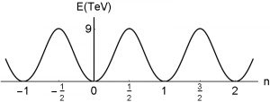
Maybe a different perspective helps to understand this important point a little better. As mentioned above, a gauge transformation always involves the generator $G_a$ and some function $f(x)$ and can be written as $U(x)=e^{i f(x) \vec{r} \vec{\sigma}}$, where $\vec{r}$ is some unit vector. The generators are just matrices and therefore the restriction $U(x)  \to 1 $ for $|x| \to \infty$ translated directly to $f(x) \to 2 \pi n$ for $|x| \to \infty$. The crucial thing is now that only these discrete endpoints are allowed for the functions that appear in the exponent of our gauge functions that satisfy $U(x)  \to 1 $ for $|x| \to \infty$. If you now imagine some arbitrary function $f(x)$ that goes to $0$ and another function $g(x)$ that goes to $2 \pi$ at spatial infinity, it becomes clear that you can’t smoothly deform $f(x)$ into $g(x)$, while keeping the endpoint fixed at one of the allowed values! The crucial thing is really that we require that endpoint at spatial infinity of the functions that appear in the exponential are restricted to the values $2 \pi n$.

Maybe an (admittedly ugly) picture helps to bring this point home:


To summarize: by restricting ourselves to a subset of gauge transformations that approach $1$ at infinity, we’re able to classify the gauge transformations according to the number which the function in the exponent approaches. This number is called the winding number and gauge transformations with a different winding number cannot be smoothly transformed into each other without leaving our subset of gauge transformations.

So far, all we found is a method to label our gauge transformations. But what does this means for our classical vacua?

We can see explicitly that two vacuum configurations that correspond to gauge transformations with a different winding number are separated by a potential barrier. This observation will mean that our infinitely many vacuum states do not lie next to each other (not meant in a spatial sense). Instead, there is a potential barrier between them.

(Afterwards, we will talk about the so-far a bit unmotivated name “winding number”.)

Origin of the Potential Barrier between Vacua

So we start with a gauge potential $A_i^{(1)}(x)$ that is generated by a gauge transformation that belongs, say, to the equivalence class with the winding number $1$. We want to describe the change of this gauge potential to the gauge potential that is generated by a gauge transformation of winding number $0$, which simply means $A_i^{(0)}=0$. A possible description is

$$  A_i^{(\beta)}(x) = \beta A_i^{(1)}(x) $$

where $\beta$ is a real parameter. For $\beta =0$, we get the gauge potential with winding number $0$: $A_i^{(0)}=0$, and for $\beta =1$, we get the gauge potential with winding number $1$:$A_i^{(1)}(x) $.

For $\beta =1$ and $\beta =0$ our $A_i^{(\beta)}(x)$ corresponds to zero classical energy, because we are dealing with a pure gauge potentials.

However, for any other value for $\beta$ in between: $0<\beta <1$, our $A_i^{(\beta)}(x)$ is not pure gauge!

The analogue of the electric field for a non-abelian gauge theory $E_i \equiv G^{0i}$ still vanishes, because$\dot{A}_i^{(\beta)}=0$ and $A_i^{(\beta)}(x)$ are time-independent. In contrast, the analogue of the magnetic field $V_i \equiv \frac{1}{2} \epsilon{ijk}G^{jk}$ does not vanish:

\begin{align}  G_{jk} &= \beta(\partial_j A_k^{(1)}-\partial_k A_j^{(1)} + \beta^2 [A_j^{(1)},A_k^{(1)} ] \notag \\
&=(\beta^2-\beta)[A_j^{(1)},A_k^{(1)} ] \notag \\
& \neq 0 \quad \text{ for } 0 <\beta < 1.
\end{align}

The energy is proportional to $\int Tr(G_{jk}G_{jk})d^3x$, and is therefore non-zero for $0< \beta < 1$. It is important to notice that it not only non-zero, but also finite. This is, because at the boundaries $A_k^{(1)}$ vanishes sufficiently fast.

To summarize: $A_i^{(\beta)}(x)$ describes the transition from a vacuum state with winding number $1$ to a vacuum state with winding number $0$. By considering the field energy $\int Tr(G_{jk}G_{jk})d^3x$, explicitly, we can see that during this transition the field does not stay in a pure gauge transformation all the time. Instead, during the transition from $A_i^{(1)}(x) $ to $A_i^{(0)}(x) $ we necessarily encounter field configurations that correspond to a non-zero, but finite, field energy. In this sense, we can say that there is a finite potential barrier between vacua with a different winding number.

What is a winding number?

In the previous sections, we simply used the notion “winding number”.  This notion is best understood by considering an easy example with $U(1)$ as a gauge group. In addition, to make things even more simple, we restrict ourselves to only one spatial dimension. Afterward, we will talk about the notion winding number in the $SU(2)$ and 4D context that we are really interested here.

Winding Number for a U(1) gauge theory

As a reminder: We are interested in gauge transformations that yield physical gauge field configurations through

\begin{equation}
G_{\mu}^{\left( pg\right) }=\frac{-i}{g(x)}U\partial_{\mu}U^{\dagger}
\end{equation}

Thus, we assume that our $g(x)$ behave nicely everywhere. Especially this means that $g(x)$ must be a continuous function because otherwise, we would have points with infinite field momentum. The reason for this is that the field momentum is directly related to the derivative of the field with respect to $x$ and if there is a non-continuous jump somewhere, the derivative of the field would be infinity there.

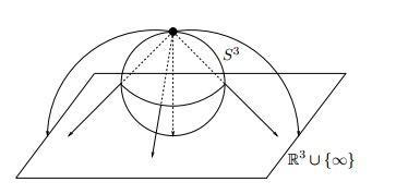
As casually mentioned above (and as will be discussed below),  we restrict ourselves to those gauge transformations $U(x)$ that satisfy $U(x) \to 1 $ for  $|x| \to \infty$.  This condition means that we are allowed to consider the range where $x$ is defined as an element of $S^1$ instead of as an element of $\mathbb{R}$. The reason for this is $U(x) \to 1 $ for  $|x| \to \infty$ means that $U(x)$ has the same value at $x= – \infty$ and at $x= \infty$. Since all that interests us here is $U(x)$ or functions that are derived from $U(x)$, we can use instead of two points $-\infty$ and $\infty$, just one point, the point at infinity.  Expressed differently, because of the condition $U(x) \to 1 $ for  $|x| \to \infty$ we can treat $x= -\infty$ and $x = \infty$ as one point and this means our $\mathbb{R}$ becomes a circle $S^1$:

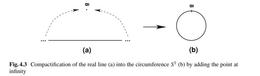
source: http://www.iop.vast.ac.vn/theor/conferences/vsop/18/files/QFT-4.pdf

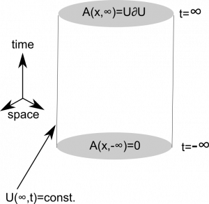
Here’s the same procedure for 3 dimensions:

Source: https://arxiv.org/pdf/hep-th/0010225.pdf

Therefore, our gauge transformations are no longer functions that eat an element of $\mathbb{R}$ and spit out an element of the gauge group $U(1)$, but instead they are now maps from the circle $S^1$ to $U(1)$. Points on the circle can be parameterized by an angle $\phi$ that runs from $0$ to $2\pi$ and therefore, we can write possible maps as follows:

$$ S^1 \to U(1) : g(\phi)= e^{i\alpha(\phi)} \, . $$

A key observation is now that the set of all possible $g(\phi)$ is divided into various topological sectors, which can be labeled by an integer $n$. This can be understood as follows:

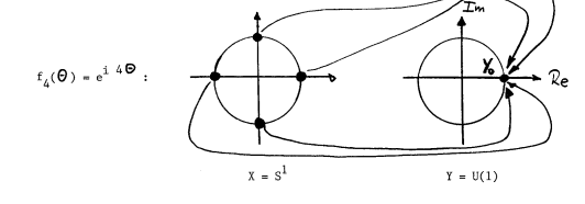
The map from the circle $S^1$ to $U(1)$ needs not to be one-to-one. The degree to which a given map is not one-to-one is the winding number. For example, when the map is two-to-one, the winding number is 2. A map from the circle onto elements of $U(1)$ is

$$ S^1 \to U(1) : f_n(\phi)= e^{in\phi} \, . $$

This map eats elements of the circle $S^1$ and spits out a $U(1)$. Now, depending on the value of $n$ in the exponent we get for multiple elements of the circle the same $U(1)$ element.

Here is how we can think about a map with winding number 1:

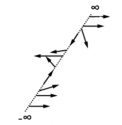
(For simplicity, space is here depicted as a line instead of a circle. Just imagine that the endpoints ∞ and -∞ are identified.)

Each arrow that points in a different direction stands for a different $U(1)$ element. As we move from ∞ to -∞ we encounter each $U(1)$ element exactly once. Similarly, a gauge transformation with winding number $0$ would only consist of arrows that point upwards, i.e. each element is mapped to the same $U(1)$ element, namely the identity. A gauge transformation with winding number 2 would consist of arrows that rotate twice as we move from ∞ to -∞, and so on for higher winding numbers.

Formulated differently, this means that depending on $n$ our map $f_n(\phi)$ maps several points on the circle onto the same $U(1)$ element.

For example, if $n=2$, we have
$$ f_2(\phi)= e^{i2\phi} .$$
Therefore
$$ f_2(\pi/2)= e^{i \pi} = -1 $$
and also
$$ f_2(3\pi/2)= e^{i3 \pi} = e^{i2 \pi} e^{i1 \pi} = -1 .$$

Therefore, as promised, for $n=2$ the map is two-to-one, because $\phi=\pi/2$ and $\phi= 3\pi/2$ are mapped onto the same $U(1)$ element. Equally, for $n=3$, we get for $\phi=\pi/3$, $\phi=\pi$ and $\phi= 5\pi/3$ the same $U(1)$ element $f_3(\pi/3)=f_3(\pi)=f_3(5\pi/3)=-1$.

In this sense, the map $f_n(\phi)$ determines how often $U(1)$ is wrapped around the circle and this justifies the name “winding number” for the number $n$.

Source: page 80 Selected Topics in Gauge Theories by Walter Dittrich, Martin Reuter


As a side remark: The elements of $U(1)$ also lie on a circle in the complex plane. ($U(1)$ is the group of the unit complex numbers). Thus, in this sense, $f_n(\phi)$ is a map from $S^1 \to S^1$.

A clever way to extract the winding number for an arbitrary map $ S^1 \to U(1)$ is to compute the following integral

$$ \int_0^{2\pi} d\phi \frac{f_n'(\phi)}{f_n(\phi)} = 2\pi i n, $$
where $f_n'(\phi)$ is the derivative of $f_n(\phi)$. Such tricks are useful for more complicated structures where the winding number isn’t that obvious.

Winding Number for an SU(2) gauge theory

Now, analogous to the compactification of $\mathbb{R}$ to the circle $S^1$, we compactify our three space dimensions to the three-sphere $S^3$. The argument is again the same, that the restriction $U(x) \to 1 $ for  $|x| \to \infty$ means that spatial infinity looks everywhere the same, no matter how we approached it (i.e. from all directions). Thus there is just one point infinity and not, for example, the edges of a hyperplane as infinities.

Thus, for a $SU(2)$ gauge theory our gauge transformations are maps from $S^3$ to $SU(2)$. In addition, completely analogous to how we can understand $U(1)$, i.e. the set of unit complex numbers, as the circle $S^1$, we can understand $SU(2)$, the set of unit quaternions, as a sphere $S^3$. Thus, in some sense our gauge transformations, are maps

$$ S^3 \to S^3 \quad : \quad U(x) = a_0(x) 1 + i a_i(x) \sigma ,$$
where $\sigma$ are the Pauli matrices.

Again, we can divide the set of all $SU(2)$ gauge transformations into topological distinct sets that are labeled by an integer.

Analogous to how we could extract the $U(1)$ winding number from a given gauge transformation, we can compute the $SU(2)$ winding number by using an integral formula (source: page 23 here):

$$n = \frac{1}{24\pi^2} \int_{S^3} d^3x \epsilon_{ijk} Tr\left[ \left( U^{-1} \partial_i U \right)\left(U^{-1} \partial_jU \right)\left(U^{-1} \partial_kU \right) \right] $$

This formula looks incredibly complicated, but can be understood quite easily.  The trick is that we can parametrize elements of $SU(2)$ by Euler angles $\alpha,\beta,\gamma$ and then define a volume element in parameter space

$$ d\mu(U) = \frac{1}{16\pi} \sin\beta d\alpha d\beta d\gamma . $$

Then by an explicit computation one can show that this volume element can be expressed as

$$d\mu(U) = \frac{1}{4\pi} Tr\left[ \left( U^{-1} \partial_i U \right)\left(U^{-1} \partial_jU \right)\left(U^{-1} \partial_kU \right) \right]d\alpha d\beta d\gamma .$$

This allows us to see that the integral over this volume element yields indeed, when we integrate $x$ all over the spatial $S^3$, the number of times we get the $SU(2)$ manifold. Moreover, geometrically $SU(2)$ is $S^3$, too. Expressed differently, when $x$ ranges one time over all points on the spatial sphere $S^3$, the winding number integral is simply the integral over the volume element of $SU(2)$ and yields the number of times we get the $SU(2)$ manifold. For example, when we have the trivial gauge function

$$U=1 ,$$

we cover the $SU(2)$ sphere zero times.

However, for example, for

$$  U^{(1)}(x) = \frac{1}{|x|}(x_4+ \vec x \cdot \vec \sigma)$$

we can see that we get exactly one time all the points of a sphere $S^3$, when the $x$ range one time over all points on the spatial $S^3$. Thus this gauge transformation has winding number $1$.

Gauge transformations with an arbitrary winding number can be computed from the gauge transformation with winding number $1$ via

$$ U(x)^{(n)} = [U^{(1)}(x)]^n $$

All this is shown nicely and explicitly on page 90 in the second edition of Quarks, Leptons and Gauge Fields by Kerson Huang.  He also shows explicitly why $ U(x)^{(n)} = [U)^{(1)}(x)]^n $ holds.

Now it’s probably time for a short intermediate summary.

Intermediate Summary – What have we learned so far?

We started by studying vacuum configurations of Yang-Mills field theory (a gauge theory, for example, with $SU(3)$ gauge symmetry like QCD). Vacuum configurations correspond to field configurations with a minimal amount of field energy. This means they correspond to vanishing field strength tensors and thus to gauge potential configurations that are pure gauge:

$$A_\mu = U \partial_\mu (U^{-1}) .$$

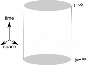
We then made two assumptions. While the first assumption (temporal gauge $A_0 = 0$) look okay, the second one is really strange: We restrict ourselves to those gauge transformations that satisfy the condition $U(x) \to 1$ for $|x| \to \infty$. Just to emphasize how strange this assumption is, here is a picture:

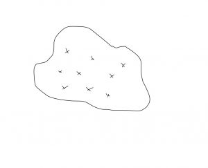
Imagine this geometrical objects represents all gauge transformations, i.e. each point is a gauge transformation. What we do with the restriction $U(x) \to 1$ for $|x| \to \infty$ is cherry picking. We pick from this huge set only a very specific set of gauge transformations, denoted by $X$’s in the picture. With this in mind, it’s no wonder that the resulting topology is non-trivial.

However, without discussing this assumption any further we pushed on and discussed the picture of the vacuum that emerges from these assumptions.

We found that the subset of all gauge configurations that satisfy $U(x) \to 1$ for $|x| \to \infty$ can be classified with the help of a label called winding number. We then computed that if the gauge potential changes from one vacuum configuration with a given winding number to a configuration with a different winding number, it needs to go through configurations that correspond to a non-zero field energy. This means that there is a potential barrier between configurations with a different winding number.

We then talked about why the name “winding number” makes sense. The crucial point is that this number really measures how often the gauge group winds around spacetime.

Physical Implications of the Periodic Structure

The first ones who came up with the periodic picture of the QCD vacuum that we described above, were Jackiw and Rebbi in 1976. However, they didn’t simply looked at QCD and then derived this structure.

Instead, they a had a very specific goal when they started their analysis. Their study was motivated by the recent discovery of so-called instantons (Alexander Belavin, Alexander Polyakov, Albert Schwarz and Yu. S. Tyupkin 1975).

Instantons are finite energy solutions of the Yang-Mills equations in Euclidean spacetime. For reasons that will be explained in a second post, this leads to the suspicion that they have something to do with tunneling processes.

(In short: The transformation from Minkowski to Euclidean spacetime is $t \to i \tau$. A “normal” wave function in quantum mechanics looks like $\Psi \sim e^{iEt}$. Now, remember how the quantum mechanical solution looks like for the tunneling of a particle through a potential barrier $\Psi \sim e^{-Et}$. The difference is $t \to i \tau$, too! This is the main reason why normal solutions in Euclidean spacetime are considered to be tunneling solutions in Minkowski spacetime.)

The motivation behind the study by Jackiw and Rebbi was to make sense of these instanton solutions in physical terms. What is tunneling? And from where to where?

(While you may not care about the history of physics, this bit of history is crucial to understand the paper by Jackiw and Rebbi; and especially how the standard picture of the QCD vacuum came about. The important thing to keep in mind is that instantons were discovered before the periodic structure of the QCD vacuum. )

The notion “winding number” was already used by Belavin, Polyakov, Schwarz, and Tyupkin. However, no physical interpretation was given. The idea by Jackiw and Rebbi was that instantons describe the tunneling between vacuum states that carry different winding number. Most importantly, they had the idea that vacuum states with different integer winding number are separated by a potential barrier, as already discussed above. Thus, the vacuum states do not lie “next to each other” and the quantum field can only transform itself from one such vacuum state into another through a tunneling process (or, of course, if it carries enough energy, for example, when the temperature is high enough).

The situation then is completely analogous to an electron in a crystal. The crystal is responsible for a periodic structure in which the electron “moves”. Like the QCD gauge field, the electron needs to tunnel to get from one minimum in the crystal potential to the next. Let’s say the minima of the crystal potential are separated by a distance $a$. Then, we can conclude that the periodic structure of the potential means that the wave function must be periodic, too: $\psi(x) = \psi(x+a)$! However, we are dealing with quantum mechanical wave functions and thus, it’s possible that the electron picks up a phase when it tunnels from one minimum to the next: $\psi(x) = e^{i\theta} \psi(x+a)$! This makes no difference for the conclusion that the probability to find the electron must be the same for locations that are separated by the distance $a$. The correct states of the electron are then not described by some $\psi(x)$, but rather by a superposition of the wave function of all minima. There are different superpositions possible, and each one is characterized by a specific value of the phase parameter $\theta$. The resulting wave function is known as Bloch wave and the phase $\theta$ as Bloch momentum. (You can read much more on this, for example in Kittel chapter 9 and Ashcroft-Mermin chapter 8).

The idea of Jackiw and Rebbi was that we have exactly the same situation for the QCD vacuum.

We have a periodic potential, tunneling between the minimas, and consequently also a parameter $\theta$, analogous to the Bloch momentum. (Take note that for the QCD vacuum neighboring minima are not separated by some distance $a$, but instead by a winding number difference of $1$.) Upon closer inspection, it turns out that the parameter $\theta$ leads to CP violation in QCD interactions and can, in principle, be measured.

It is important to know the backstory of the paper by Jackiw and Rebbi because otherwise some of their arguments do not seem to make much sense. They already knew about the instanton solutions and had the “electron in a crystal” picture in mind as a physical interpretation of the instantons. Around this idea, they wrote their paper.

The periodic vacuum structure of the QCD vacuum was not discovered from scratch, but with these very specific ideas in mind.

We have seen above, that the periodic structure of the QCD vacuum does not arise without two crucial assumptions. If you know that this structure was first described with instantons and Bloch waves in mind, it makes a lot more sense how the original authors came up with these assumptions. These assumptions are exactly what you need to give the QCD vacuum the nice periodic structure and thus to be able to draw the analogy with an electron in a crystal. As I will describe in a later post, without these assumptions, the QCD vacuum looks very different.

In their original paper, Jackiw and Rebbi motivated one of the assumptions, namely the restriction to gauge transformations that satisfy $g(x) \to 1$ for $|x| \to \infty$, simply with “we study effects which are local in space and therefore”. As far as I know, this reason does not make sense and was never again repeated in any later paper. In subsequent papers, Jackiw came up with all sorts of different reasons for this restriction. However, ultimately in 1980, he concluded: “while some plausible arguments can be given in support of this hypothesis (see below) in the end we must recognize it as an assumption” (Source).

The path to the standard periodic picture of the QCD vacuum was thus not through some rigorous analyses, but rather strongly guided by “physical intuition”. It was the idea, that the interpretation of the QCD vacuum could be done similar to the quantum mechanical problem of an electron in a crystal, which lead to the periodic picture of the QCD vacuum.

My point is not that this picture is wrong. Instead, I was long puzzled for along time by the reasons that are given for the restriction $g(x) \to 1$ for $|x| \to \infty$ and I want to help others who are confused by them, too. I will write a lot more about this in a second post, but I hope that the few paragraphs above already help a bit. The path to the periodic vacuum structure is not as straight-forward as most authors want you to believe. However, it is important to keep in mind that only because physicists came up with a description through intuition and not via some rigorous analysis, does not mean that it is wrong. Even when the original arguments the discoverers give do not hold upon closer scrutiny, it is still possible that their conclusions are correct. As already mentioned above, after the original publication, both Jackiw and Rebbi and many other authors, came up with lots of other arguments to strengthen the case for the periodic vacuum picture.

However, it is also important to keep in mind that, so far, all experimental evidence point in the direction that $\theta$ is tiny $\theta \lesssim 10^{10}$ or even zero. This is hard to understand if you believe in the analogy with the Bloch wave. In this picture, $\theta$ is an arbitrary phase and could be any value between $0$ and $2\pi$. There is no reason why it should be so tiny or even zero. This is famously known as the strong CP problem. (Things aren’t really that simple. The parameter $\theta$ also pops up from a completely different direction, namely from an analysis of the chiral anomaly. Thus, even if you don’t believe in the Bloch wave picture of the QCD vacuum, you end up with a $\theta$ parameter. Much more on this in a later post.)

Outlook (or: which puzzle pieces are still missing?)

Unfortunately, there are still a lot of loose ends. These will be hopefully tied up in future posts.

Most importantly we need to talk more about the assumptions

1.) The choice of the temporal gauge $A_0 = 0$.
2.) The restriction to those gauge transformations that become trivial at infinity $U(x) \to 1$ for $|x| \to \infty $.

In the second post of this series, I will try to elucidate these assumptions which are only noted in passing in almost all standard discussion of the QCD vacuum.

In a third post, I will show how the QCD vacuum can be understood beautifully from a completely different perspective.

Another important loose end is that we have not talked about instantons so far. These are solutions of the Yang-Mills equations and describe the tunneling processes between degenerate vacua.

Until I have finished these posts, here are some reading recommendations.

Reading Recommendations

The classical papers that elucidated the standard picture of the QCD vacuum are:

  • Vacuum Periodicity in a Yang-Mills Quantum Theory by R. Jackiw and C. Rebbi
  • Toward a theory of the strong interactions by Curtis G. Callan, Jr., Roger Dashen, and David J. Gross
  • The Structure of the Gauge Theory Vacuum Curtis G. Callan et. al.
  • Pseudoparticle solutions of the Yang-Mills equations A.A. Belavin et. al.
  • Concept of Nonintegrable Phase Factors and Global Formulation of Gauge Fields Tai Tsun Wu (Harvard U.), Chen Ning Yang

The standard introductions to instantons and the QCD vacuum are:

  • ABC of instantons by A I Vaĭnshteĭn, Valentin I Zakharov, Viktor A Novikov and Mikhail A Shifman
  • The Uses of Instantons by Sidney Coleman

(However, I found them both to be not very helpful)

Books on the topic are:

  • The QCD Vacuum, Hadrons and Superdense Matter by E. V. Shuryak
  • Solitons and Instantons by Ramamurti Rajaraman (Highly Recommended)
  • Classical Solutions in Quantum Field Theory: Solitons and Instantons by Erick Weinberg
  • Topological Solitons by Manton and Sutcliff (Highly Recommended)
  • Some Elementary Gauge Theory Concepts Hong-Mo Chan, Sheung Tsun Tsou
  • Classical Theory of Gauge Fields by Rubakov (Highly Recommended)

Review articles are:

  • Theory and phenomenology of the QCD vacuum by Edward V. Shuryak
  • A Primer on Instantons in QCD by Hilmar Forkel (Highly Recommended)
  • Effects of Topological Charge in Gauge Theories R.J. Crewther
  • TASI Lectures on Solitons Instantons, Monopoles, Vortices and Kinks David Tong
  • Topological Concepts in Gauge Theories by F. Lenz

Textbooks that contain helpful chapters on instantons and the QCD vacuum are:

  • Quarks, Leptons & Gauge Fields by Kerson Huang (Highly Recommended)
  • Quantum Field Theory by Lewis H. Ryder (Highly Recommended)
  • Quantum Field Theory by Mark Srednicki (Highly Recommended)
  • Quantum Field Theory and Critical Phenomena by Zinn-Justin

Another informal introduction is:

  • ’t Hooft and η’ail Instantons and their applications by Flip Tanedo

The same things explained more mathematically can be found in:

  • Geometry of Yang-Mills Fields by M. F. ATIYAH
  • plus chapters in Geometry of Physics by Frankel and
  • Topology and Geometry for Physicists by Nash and Sen