In this post I discussed why the gauge couplings depend on the energy scale. Here I discuss how we can compute this change with energy in practice. This is another post from the category “I wished this kind of post had existed when I started”. In addition to the general formulas, I discuss two examples in detail. Moreover, I list numerical values for the group invariants that apear in the general formulas at the end of this post.

The RGEs for a gauge coupling constant depend on the particles that can appear in the loops as virtual pairs and therefore contribute to the screening of the charge. Luckily there are general formulas that we can use to derive the $\beta$-functions for a given particle content. Defining $\omega_i := \alpha_i^{-1} := \frac{4\pi}{g_i^2}$ and denoting the coupling strength corresponding to the gauge group $i$ by  $g_i$, we have up to $2$-loop order

\begin{equation}
\mu \frac{d\omega_i(\mu)}{d  \mu}=-\frac{a_i}{2 \pi} – \sum_j \frac{b_{ij}}{8\pi^2\omega_j(\mu)} \,.
\end{equation}

This can be written in a more compact form using $ \frac{d\ln(\mu)}{d \mu}  = \frac{1}{\mu} \rightarrow d\ln(\mu) = \frac{d\mu}{\mu} $

\begin{equation} \label{eq:gaugerges}
\frac{d\omega_i(\mu)}{d \ln(\mu)}=-\frac{a_i}{2 \pi} – \sum_j \frac{b_{ij}}{8\pi^2\omega_j(\mu)} \, .
\end{equation}

The numbers $a_i$ are called 1-loop beta coefficients and $b_{ij}$ the 2-loop beta coefficients For a $G_1 \times G_2$ gauge group they are given by

\begin{equation} \label{eq:1LoopRGE}
a_i = \frac{2}{3}T(R_1)d(R_2)+ \frac{1}{3} T(S_1)d(S_2) -\frac{11}{3}C_2(G_1) \,.
\end{equation}

The generalization to $G_1 \otimes G_2 \otimes \ldots$ will be explained using an explicit example in the next section.

The $2-$loop beta coefficients for $i=j$ are given by

\begin{equation} \label{eq:2LoopRGEii}
b_{ij} = \Big(\frac{10}{3} C_2(G_1)+2C_2(R_1) \Big) T(R_1)d(R_2)+ \Big(\frac{2}{3} C_2(G_1)+4C_2(S_1) \Big) T(S_1) d(S_2)- \frac{34}{3} (C_2(G_1))^2
\end{equation}

and for $i \neq j$

\begin{equation} \label{eq:2LoopRGEij}
b_{ij} = 2C_2(R_2)d(R_2)T(R_1)+4C_2(S_2)d(S_2)T(S_1)\, .
\end{equation}

As noted above our gauge group is $G_1 \otimes G_2$. The fermions representation is denoted by $(R_1,R_2)$ and the scalar representation by $(S_1,S_2)$. The other symbols that appear in the equations are:

• $T(R_i)$, which denotes the Dynkin index of the representation $R_i$
• $T(S_i)$, which denotes the Dynkin index of the representation $S_i$
• $C_2(R_i)$, which denotes the quadratic Casimir operator of the representation $R_i$
• $C_2(S_i)$, which denotes the quadratic Casimir operator of the representation $S_i$
• $C_2(G_i)$, which denotes the quadratic Casimir operator of the group $G_i$ which is defined as the quadratic Casimir operator of the adjoint representation of $G_i$
• $d(R_i)$ the dimension of the representation $R_i$
• $d(S_i)$ the dimension of the representation $S_i$.

If the fermions (or scalars) live in a reducible representation, e.g. $(R_1^1,R_2^1) \oplus (R_1^2,R_2^2)$, the contributions from both irreducible representations get added and in general we sum over all irreducible representations. For the $a_i$ formula this means we have $\frac{2}{3}T(R_1^1)d(R_2^1) +\frac{2}{3}T(R_1^2)d(R_2^2)$. Further one must keep in mind that in most realistic models we are dealing with $3$ generations of fermions and therefore the fermionic part in the equations gets multiplied by three. In other words, three generations means we have $(R_1^1,R_2^1) \oplus (R_1^2,R_2^2)\oplus (R_1^3,R_2^3)$, but the three irreducible representations are identical with respect to the gauge group and therefore we can simply multiply by three. For the $a_i$ this means explicitly $\frac{2}{3}T(R_1^1)d(R_2^1)\cdot 3$ for each fermion representation. The relevant group invariants are listed at the end of this post. We will discuss two explicit examples in a moment, but there is one importang thing we must take into account.

Normalization of the Hypercharge

There is one subtlety when one of the groups in the product $G_1 \otimes G_2$ is $U(1)$. For example, this is the case for the standard model gauge group $SU(3) \times SU(2) \times U(1)$. In the standard model the normalization of the $U(1)$ charges (the hypercharges) are not fixed. We can always rescale $ Y \equiv a Y’$ and absorb the extra factor $a$ into the coupling constant $g_Y \equiv \frac{g_Y’}{a}$. Any normalization choice is equally good.  This is a strange situation, because the RGEs depend on the hypercharges. This means, the running of the standard model $U(1)$ depends on the normalization that we choose for the hypercharges. This means, for example, we could always rescale our hypercharge such that the three coupling constants meet at a point: $g_{2L}$ and $g_{3C}$ must meet somewhere if their running is not completely equal. Then we can rescale our hypercharges, which changes the starting point of $g_Y$, such that $g_Y$ intersects this point, too. However, if the standard model gauge group is interpreted as a remnant of a broken unification group, there is only one correct normalization and no ambiguity.

When we embed $G_{SM}$ in a larger gauge group $G_{GUT}$, we no longer have the freedom to rescale. In such scenarios the $U(1)_Y$ generator must correspond to a generator of the enlarged gauge symmetry and therefore its normalization must be the same as for the other generators. The normalization of the generators of a non-abelian group is fixed through the Dynkin index of the fundamental representation $T(f)= c$, where the most common convention is $c=\frac{1}{2}$. (A notable exception is Slansky, who uses the convention $c=1$.) The Dynkin index of a representation is defined in the last section of this post.

For example if $G_{SM}$ is embedded in $SU(5)$, one usually identifies the components of the conjugate $5$-dimensional representation as the anti-right-handed down quark and the left-handed lepton doublet. Therefore under $SU(3) \times SU(2) \times U(1)$, we have the decomposition

\begin{align}
\bar{5} = (1, \bar 2)_{-\frac{1}{2}a} \oplus (\bar{3},1)_{\frac{1}{3}a} = \begin{pmatrix} \nu_L \\ e_L \end{pmatrix} \oplus \begin{pmatrix} (d_R^c)_{\text{r}} \\ (d_R^c)_{\text{b}} \\ (d_R^c)_{\text{g}} \end{pmatrix} = \begin{pmatrix} \nu_L \\ e_L \\ (d_R^c)_{\text{r}} \\ (d_R^c)_{\text{b}} \\ (d_R^c)_{\text{g}} \end{pmatrix}
\end{align}

The relative factors $-\frac{1}{2}$ and $\frac{1}{3}$ for the $U(1)$ charge are fixed, because here Cartan generators are diagonal $5\times 5$ matrices with trace zero\footnote{Recall that $SU(5)$ is the set of $5 \times 5$ matrices $U$ with determinant $1$ that fulfil $U^\dagger U = 1$. For the generators $T_a$ this means $\text{det}(e^{i \alpha_a T_a})=e^{i \alpha_a Tr(T_a)} \stackrel{!}{=}1$. Therefore  $Tr(T_a) \stackrel{!}{=} 0$}. Therefore we have
\begin{align}
&Tr(Y)= Tr \begin{pmatrix} Y(\nu_L) & 0 & 0 & 0 &0 \\  0 & Y(e_L) & 0 & 0 &0 \\ 0 & 0 & Y((d_R^c)_{\text{r}}) & 0 &0\\ 0 & 0 & 0 & Y((d_R^c)_{\text{b}})&0\\ 0 & 0 & 0 & 0 &Y((d_R^c)_{\text{g}}) \end{pmatrix} \stackrel{!}{=} 0 \notag \\
&\rightarrow 2 Y(L)  + 3Y(d_R^c) \stackrel{!}{=} 0
\end{align}

This means the hypercharge generator in $SU(5)$ models reads\footnote{$\nu_L$ and $e_L$ must have the same hypercharge $Y(L)$, because they live in a $SU(2)$ doublet after the breaking of the $SU(5)$ symmetry.}
\begin{equation}
Y=
\begin{pmatrix} -\frac{1}{2}a & 0 & 0 & 0 &0 \\  0 & -\frac{1}{2}a & 0 & 0 &0 \\ 0 & 0 & \frac{1}{3}a & 0 &0\\ 0 & 0 & 0 & \frac{1}{3}a&0\\ 0 & 0 & 0 & 0 &\frac{1}{3}a \end{pmatrix} \, .
\end{equation}

Demanding that the Dynkin index of this generator in the fundamental representation is $\frac{1}{2}$ yields

\begin{align}
T(\bar{5}) &=  Tr(Y^2)  \stackrel{!}{=} \frac{1}{2} \notag \\
& \rightarrow \frac{5}{6} a^2 = \frac{1}{2} \notag \\
& \rightarrow a = \sqrt{\frac{3}{5}} \, .
\end{align}

Completely analogous we compute that the hypercharge normalization in $SO(10)$ models is $a = \sqrt{\frac{3}{5}}$, too.

To summarize: The correct normalization is given by

\begin{equation}Y’ = \sqrt{\frac{3}{5}} Y ,\end{equation}

where $Y$ is the usual hypercharge and $Y’$ the correctly normalized hypercharge that must be used when we evaluate the RGEs.

Take note that if there is more than $U(1)$ subgroup at some intermediate scale, there are further subtleties one must take into account. For example, the definitions of the $U(1)$ subgroups can not be chosen arbitrarily and a wrong choice yields a wrong unification scale. This is illustrated nicely in this paper. Therefore one must be careful which definition is used for the RGE running. A recent discussion how this is done correctly can be found here.

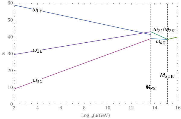
Explicit Example: $SU(4) \times SU(2) \times SU(2) \times D$  $1-$Loop Beta Coefficients

Consider a theory with gauge group $SU(4) \times SU(2)_R \times SU(2)_L \times D$, where $D$ denotes $D$-parity, which is a discrete symmetry that exchanges $L \leftrightarrow R$. We have three generations of fermions in $(4,1,2)\oplus(\bar{4},2,1)$ plus scalars in $(1,2,2)\oplus (10,3,1) \oplus (\overline{10},1,3) $. Here $G_1$ is the group whose coupling constant we are considering.  Using Eq. \ref{eq:1LoopRGE} we have (here, $SU(4)$ is $G_1$, $SU(2)_R$ is $G_2$ and $SU(2)_L$ is $G_3$. Therefore $R_1$, $S_1$ denote the corresponding $SU(4)$ representations)

\begin{align}
a_{SU(4)} &= \frac{2}{3} (
\underbrace{\frac{1}{2}}_{T(R_1=4)} \underbrace{1}_{d(R_2=1)}\underbrace{2}_{d(R_3=2)}
+\underbrace{\frac{1}{2}}_{T(\bar{4})}\underbrace{2}_{d(R_2=2)}
\underbrace{1}_{d(R_3=1)}
)\cdot \overbrace{3}^{3 \text{ generations}} \notag \\
&\quad+ \frac{1}{3} (
\underbrace{3}_{T(S_1=10)} \cdot \underbrace{1}_{d(S_2=1)} \underbrace{3}_{d(S_3=3)}
+\underbrace{0}_{T(S_1=1)} \cdot \underbrace{2}_{d(S_2=2)} \underbrace{2}_{d(S_3=2)}
+\underbrace{3}_{T(S_1=10)} \cdot \underbrace{3}_{d(S_2=3)} \underbrace{1}_{d(S_3=1)} ) \notag \\
&\quad-\frac{11}{3} \underbrace{4}_{C_2(SU(4))} \notag \\ &
= -\frac{14}{3} \, ,
\end{align}

and (here, $SU(2)_R$ is $G_1$, $SU(4)$ is $G_2$ and $SU(2)_L$ is $G_3$. Therefore $R_1$, $S_1$ denote the corresponding $SU(2)_R$ representations)

\begin{align}
a_{SU(2)_R} &= \frac{2}{3} (
\underbrace{0}_{T(R_1=1)} \underbrace{4}_{d(R_2=4)}\underbrace{2}_{d(R_3=2)}
+\underbrace{\frac{1}{2}}_{T(R_1=2)}\underbrace{4}_{d(R_2=4)}
\underbrace{1}_{d(R_3=1)}
)\cdot \overbrace{3}^{3 \text{ generations}} \notag \\
&\quad+
\frac{1}{3} (
\underbrace{2}_{T(S_1=3)} \cdot \underbrace{10}_{d(S_2=10)} \underbrace{1}_{d(S_3=1)}  +\underbrace{\frac{1}{2}}_{T(S_1=2)} \cdot \underbrace{1}_{d(S_2=1)} \underbrace{2}_{d(S_3=2)}
+\underbrace{0}_{T(S_1=1)} \cdot \underbrace{10}_{d(S_2=10)} \underbrace{3}_{d(S_3=3)})   \notag\\
&\quad-\frac{11}{3} \underbrace{2}_{C_2(SU(2)_R)}  \notag \\ &
= \frac{11}{3} \, ,
\end{align}

and (here, $SU(2)_L$ is $G_1$, $SU(4)$ is $G_2$ and $SU(2)_R$ is $G_3$. Therefore $R_1$, $S_1$ denote the corresponding $SU(2)_L$ representations)

\begin{align}
a_{SU(2)_L} &= \frac{2}{3} (
\underbrace{\frac{1}{2}}_{T(R_1=2)} \underbrace{4}_{d(R_2=4)}\underbrace{1}_{d(R_3=1)}
+\underbrace{0}_{T(R_1=1)}\underbrace{4}_{d(R_2=4)}
\underbrace{2}_{d(R_3=2)}
)\cdot \overbrace{3}^{3 \text{ generations}} \notag \\
&\quad+
\frac{1}{3} (
\underbrace{0}_{T(S_1=1)} \cdot \underbrace{10}_{d(S_2=10)} \underbrace{3}_{d(S_3=3)}
+\underbrace{\frac{1}{2}}_{T(S_1=2)} \cdot \underbrace{1}_{d(S_2=1)} \underbrace{2}_{d(S_3=2)}
\underbrace{3}_{T(S_1=10)}
+ \underbrace{2}_{T(S_1=3)} \cdot \underbrace{10}_{d(S_2=10)} \underbrace{1}_{d(S_3=1)}
) \notag \\
&\quad-\frac{11}{3} \underbrace{2}_{C_2(SU(2)_L)} \notag \\
&= \frac{11}{3} \, ,
\end{align}

in accordance with the results in this paper.

Explicit Example: $SU(4) \times SU(2)_R \times SU(2)_L \times D$  $2-$Loop Beta Coefficients

Using Eq. \ref{eq:2LoopRGEii}, we have for the $2$-loop beta coefficients

\begin{align}
b_{SU(4)SU(4)} &=
\Big(\frac{10}{3} \underbrace{4}_{C_2(G_1=SU(4))}
+2\underbrace{\frac{3}{2}}_{C_2(R_1=4)}
\Big) \underbrace{\frac{1}{2}}_{T(R_1=4)}\underbrace{1}_{d(R_2)=1} \underbrace{2}_{d(R_3)=2} \cdot \underbrace{3}_{3 \text{ generations}} \notag \\
&\quad +\Big(\frac{10}{3} \underbrace{4}_{C_2(G_1=SU(4))}
+2\underbrace{\frac{3}{2}}_{C_2(R_1= \bar{4})}
\Big) \underbrace{\frac{1}{2}}_{T(R_1=4)}\underbrace{2}_{d(R_2)=2} \underbrace{1}_{d(R_3)=1} \cdot \underbrace{3}_{3 \text{  generations}} \notag \\
& \quad + \Big(\frac{2}{3} \underbrace{4}_{C_2(G_1=SU(4))}
+4\underbrace{\frac{9}{2}}_{C_2(S_1=10)} \Big) \underbrace{3}_{T(S_1=10)} \underbrace{3}_{d(S_2=3)} \underbrace{1}_{d(S_3=1)} \notag \\
& \quad + \Big(\frac{2}{3} \underbrace{4}_{C_2(G_1=SU(4))}
+4\underbrace{\frac{9}{2}}_{C_2(S_1=10)} \Big) \underbrace{3}_{T(S_1=10)} \underbrace{1}_{d(S_2=1)} \underbrace{3}_{d(S_3=3)} \notag \\
& \quad + \Big(\frac{2}{3} \underbrace{4}_{C_2(G_1=SU(4))}
+4\underbrace{0}_{C_2(S_1=1)} \Big) \underbrace{0}_{T(S_1=1)} \underbrace{2}_{d(S_2=2)} \underbrace{2}_{d(S_3=2)} \notag \\
& \quad – \frac{34}{3} (\underbrace{4}_{C_2(G_1=SU(4))})^2  \notag \\
&= \frac{1749}{6} \, ,
\end{align}

\begin{align}
b_{SU(2_L)SU(2_L)} = b_{SU(2_R)SU(2_R)} &=
\Big(\frac{10}{3} \underbrace{2}_{C_2(G_1=SU(2))}
+2\underbrace{\frac{3}{4}}_{C_2(R_1=2)}
\Big) \underbrace{\frac{1}{2}}_{T(R_1=2)}\underbrace{4}_{d(R_2)=4} \underbrace{1}_{d(R_3)=1} \cdot \underbrace{3}_{3 \text{  generations}}  \notag \\
&\quad +\Big(\frac{10}{3} \underbrace{2}_{C_2(G_1=SU(2))}
+2\underbrace{0}_{C_2(R_1= 1)}
\Big) \underbrace{0}_{T(R_1=1)}\underbrace{4}_{d(R_2)=\bar{4}} \underbrace{2}_{d(R_3)=2} \cdot \underbrace{3}_{3 \text{ generations}} \notag \\
& \quad + \Big(\frac{2}{3} \underbrace{2}_{C_2(G_1=SU(2))}
+4\underbrace{2}_{C_2(S_1=3)} \Big) \underbrace{2}_{T(S_1=3)} \underbrace{10}_{d(S_2=10)} \underbrace{1}_{d(S_3=1)} \notag \\
& \quad + \Big(\frac{2}{3} \underbrace{2}_{C_2(G_1=SU(2))}
+4\underbrace{0}_{C_2(S_1=1)} \Big) \underbrace{0}_{T(S_1=1)} \underbrace{10}_{d(S_2=10)} \underbrace{3}_{d(S_3=3)} \notag \\
& \quad + \Big(\frac{2}{3} \underbrace{2}_{C_2(G_1=SU(2))}
+4\underbrace{\frac{3}{4}}_{C_2(S_1=2)} \Big) \underbrace{\frac{1}{2}}_{T(S_1=2)} \underbrace{1}_{d(S_2=1)} \underbrace{2}_{d(S_3=2)} \notag \\
& \quad – \frac{34}{3} (\underbrace{2}_{C_2(G_1=SU(2))})^2 \notag \\
&= \frac{584}{3}
\end{align}

and for $i \neq j$ using Eq. \ref{eq:2LoopRGEij}

\begin{align}
b_{SU(4)SU(2)_L} = b_{SU(4)SU(2)_R} &=
2 \underbrace{\frac{3}{4}}_{C_2(R_2=2)}\underbrace{2}_{d(R_2=2)}\underbrace{\frac{1}{2}}_{T(R_1=4)} \cdot \underbrace{3}_{3 \text{ generations}} \notag \\
&\quad + 2 \underbrace{0}_{C_2(R_2=1)}\underbrace{1}_{d(R_2=1)}\underbrace{\frac{1}{2}}_{T(R_1=\bar{4})} \cdot \underbrace{3}_{3 \text{  generations}} \notag \\
& \quad +4\underbrace{0}_{C_2(S_2=1)}\underbrace{1}_{d(S_2=1)}\underbrace{3}_{T(S_1=10)} \notag \\
& \quad +4\underbrace{2}_{C_2(S_2=3)}\underbrace{3}_{d(S_2=3)}\underbrace{3}_{T(S_1=10)} \notag \\
& \quad +4\underbrace{\frac{3}{4}}_{C_2(S_2=2)}\underbrace{2}_{d(S_2=2)}\underbrace{0}_{T(S_1=1)} \notag \\
&= \frac{153}{2} \, ,
\end{align}

\begin{align}
b_{SU(2)_LSU(4)} = b_{SU(2)_RSU(4)} &=
2 \underbrace{\frac{15}{8}}_{C_2(R_2=4)}\underbrace{4}_{d(R_2=4)}\underbrace{\frac{1}{2}}_{T(R_1=2)} \cdot \underbrace{3}_{3 \text{  generations}} \notag \\
&\quad + 2 \underbrace{\frac{15}{8}}_{C_2(R_2=\bar{4})}\underbrace{4}_{d(R_2=\bar{4})}\underbrace{0}_{T(R_1=1)} \cdot \underbrace{3}_{3 \text{  generations}} \notag \\
& \quad +4\underbrace{\frac{9}{2}}_{C_2(S_2=10)}\underbrace{10}_{d(S_2=10)}\underbrace{2}_{T(S_1=3)} \notag \\
& \quad +4\underbrace{\frac{9}{2}}_{C_2(S_2=10)}\underbrace{10}_{d(S_2=10)}\underbrace{0}_{T(S_1=1)} \notag \\
& \quad +4\underbrace{0}_{C_2(S_2=1)}\underbrace{1}_{d(S_2=1)}\underbrace{\frac{1}{2}}_{T(S_1=2)}  \notag \\
&= \frac{756}{2} \, ,
\end{align}

\begin{align}
b_{SU(2)_L SU(2)_R} = b_{SU(2)_RSU(2)_L} &=
2 \underbrace{\frac{1}{2}}_{C_2(R_2=2)}\underbrace{2}_{d(R_2=2)}\underbrace{0}_{T(R_1=1)} \cdot \underbrace{3}_{3 \text{ \ generations}} \notag  \\
&\quad + 2 \underbrace{0}_{C_2(R_2=1)}\underbrace{1}_{d(R_2=1)}\underbrace{\frac{1}{2}}_{T(R_1=2)} \cdot \underbrace{3}_{3 \text{ generations}}  \notag \\
& \quad +4\underbrace{0}_{C_2(S_2=1)}\underbrace{1}_{d(S_2=1)}\underbrace{2}_{T(S_1=3)} \notag \\
& \quad +4\underbrace{2}_{C_2(S_2=3)}\underbrace{3}_{d(S_2=3)}\underbrace{0}_{T(S_1=1)} \notag \\
& \quad +4\underbrace{\frac{3}{4}}_{C_2(S_2=2)}\underbrace{2}_{d(S_2=2)}\underbrace{\frac{1}{2}}_{T(S_1=2)} \notag \\
&= 3
\end{align}

in accordance with the results in this paper.

Appendix: Group Invariants

One possibility to label representations is given by operators constructed from the generators known as Casimir operators. These are defined as those operators that commute with all generators. There is always a quadratic Casimir operator

\begin{equation}
C_2(r) = T^A T^A \, ,
\end{equation}

where $T^A$ denotes the $d(r) \times d(r)$ matrices that represent the generators in the representation $r$. Another important label is the Dynkin index, which is defined as

\begin{equation}
T(r) \delta^{AB} = \text{Tr}(T^AT^B) \, .
\end{equation}

The standard convention is that the fundamental representation has Dynkin index $\frac{1}{2}$. (Huge lists of Dynkin indices can be found in Slansky’s famous paper. However the indices listed there must be divided by $2$ because the Slansky uses the non-standard convention that the fundamental representation has Dynkin index $1$. )

The Dynkin Index of a representation and the corresponding quadratic Casimir operator are related through

\begin{equation} \label{eq:DynkinCasimirRelation}
\frac{T(r)}{d(r)}= \frac{C_2(r)}{D},
\end{equation}

where $D$ denotes the dimension of the adjoint representation, i.e. of the Lie algebra. For the adjoint representation we therefore have $T(\text{adjoint})=C_2(\text{adjoint})$.

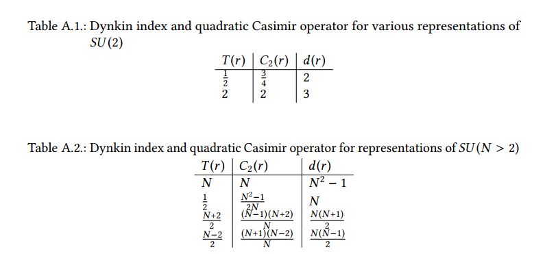
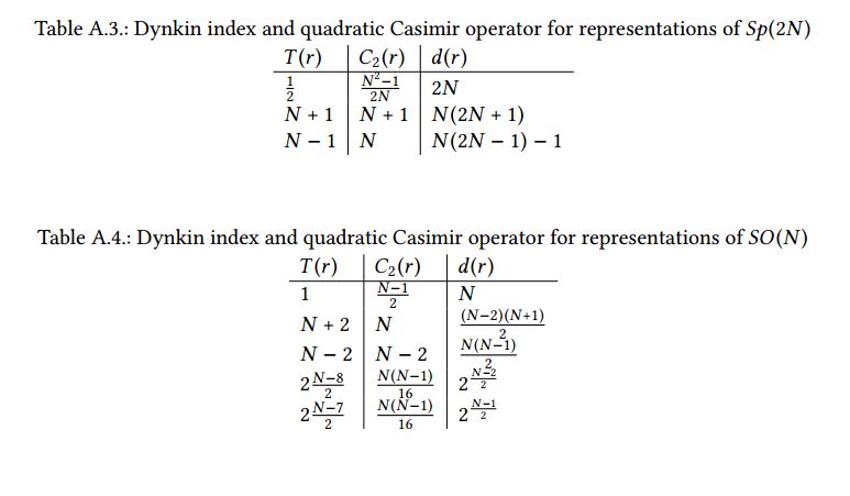
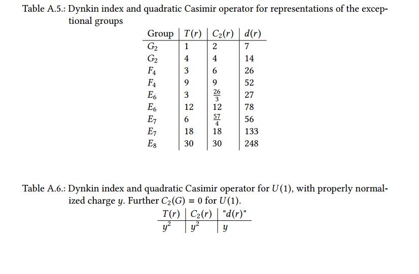
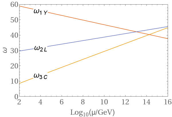
The following tables list the quadratic Casimir operators and Dynkin indices for the most important representations.

The standard model contains three gauge couplings, which are very different in strength. This is not really a problem of the standard model, because we can simply put these measured values in by hand. However, Grand Unified Theories (GUTs) provide a beautiful explanation for this difference in strength. A simple group $G_{GUT}$ implies that we have only one gauge coupling as long as $G_{GUT}$ is unbroken. The gauge symmetry $G_{GUT}$ is broken at some high energy scale in the early universe. Afterwards, we have three distinct gauge couplings with approximately equal strength. The gauge couplings are not constant, but depend on the energy scale. This is described by the renormalization group equations (RGEs).

The RGEs for a gauge coupling depend on the number of particles that carry the corresponding charge. (This is discussed in detail below.) Therefore, we can use the known particle content of the standard model to compute how the three couplings change with energy. This is shown schematically in the figure below.

The couplings change differently with energy, because the number of particles that carry, for example, color ($SU(3)$ charge) or isospin ($SU(2)$ charge) are different. The known particle content of the standard model and the hypothesis that there is one unified coupling at high energies therefore provide a beautiful explanation why strong interactions are strong and weak interactions are weak.

This is not just theory. For example, the strong coupling “constant” $\alpha_S$ has been measured at very different energy scales. Some of these measurements are summarized in the following plot.

This is figure is from Measurement of the inclusive 3-jet production differential cross section in proton-proton collisions at 7 TeV and determination of the strong coupling constant in the TeV range by the CMS Collaboration

To understand how all this comes about, recall that in quantum field theory we have a cloud of virtual particle-antiparticle pairs around each particle. This situation is similar to the classical situation of an electron inside a dielectric medium. Through the presence of the electron, the electrical neutral molecules around it get polarized, which is illustrated in the figure below. As a result, the electrical charge of the electron gets partially hidden or screened. This is known as dielectric screening.

Analogous to what happens in a dielectric medium, the virtual particle-antiparticle pairs get polarized and the charge of the particle screened. Concretely this means if we are close to a particle, we measure a different charge than from far away because there are fewer virtual particle-antiparticle pairs that screen the charge. This screening effect happens not only for electrical charge but for color-charge and weak-isospin, too. In particle physics, the notion of distance is closely related to the notion of energy. If we shoot a particle with lots of energy onto an electron it comes closer to the electron before it gets deflected than a particle with less energy. Therefore, the particle with more energy feels a larger charge. It may now seem that our three coupling strengths all get bigger if we measure them at higher energies. However, it turns out that gauge bosons have the opposite effect than fermions. They anti-screen and thus make a given charge bigger at larger distances. Recall that we have:

• One gauge boson for $U(1)$.
• Three gauge bosons for $SU(2)$, because the adjoint representation is $3$-dimensional.
• Eight gauge bosons for $SU(3)$, because the adjoint representation is $8$-dimensional.

These numbers tell us that $SU(3)$ couplings are more affected by the gauge boson anti-screening effect, simply because there are more $SU(3)$ gauge bosons. In fact, it can be computed that their effect outweighs the screening effect of the quarks and thus the $SU(3)$ coupling constant gets weaker at smaller distances. For $SU(2)$ the gauge boson and fermion effect is almost equal and therefore the coupling strength is approximately constant. For $U(1)$ the ordinary screening effect dominates and the corresponding coupling strength becomes stronger at smaller distances.  Given the coupling strengths at some energy scale, we can compute at which energy scale they become approximately equal.

This energy scale is closely related to the mass of the GUT gauge bosons $m_X$. From an effective field theory point of view, at energies much higher than $m_X$ the breaking of the GUT symmetry has a negligible effect and therefore the gauge coupling constants unify. The mathematical description of this coupling strength change with energy, known as renormalization group equations, is the topic of the next section. The coupling constants change so slowly with the energy that the scale where they are approximately equal is incredibly high. This means the GUT gauge bosons are so heavy that it is no wonder they have not been seen in experiment yet.

The Renormlization Group Equations

To illustrate the arguments that lead to the famous renormalization group equations, we discuss shortly the arguably simplest example in quantum field theory: the Coulomb potential $ V(r) =\frac{e^2}{4 \pi r}$. In QFT it corresponds to the exchange of a single photon

and $\frac{1}{4 \pi r}$ is the Fourier transform of the propagator. A $1$-loop correction to this diagram is, for example,

which yields a correction of order $e^4$ to the Coulomb potential. In momentum space, the Coulomb potential then reads

\begin{equation}
\tilde{V}(p)=e^2 \frac{1-e^2 \Pi_2(p^2)}{p^2},
\end{equation}
where $\Pi_2(p^2) = \frac{1}{2\pi^2} \int_0^1 dx \, x(1-x)\left[ \frac{2}{\epsilon} + \ln \left(\frac{\tilde{\mu}^2}{m^2-p^2x(1-x)}\right) \right]$ (see for example the QFT book by Schwartz or the similar free chapter here). The usual problem in QFT is now that $\Pi_2(p^2)$ is infinite and we need to renormalize. For this reason, we demand that the potential between two particles separated by some distance $r_0$ should be $V(r_0) = \frac{e_R^2}{2\pi r_0}$, where $e_R$ denotes the renormalized charge. In momentum space this means $\tilde{V}(p_0)=\frac{e_R^2}{p_0^2}$. This defines the renormalized charge

\begin{equation}
e_R^2 := p_0^2 \tilde{V}(p_0) = e^2- e^4 \Pi_2(p^2) + \ldots \, ,
\end{equation}

where the dots denote higher order corrections. Equally, we can solve for the bare charge
\begin{equation} \label{eq:defbarecharge}
e^2 := e_R^2+e_R^4 \Pi_2(p_0^2) + \ldots
\end{equation}

At another momentum scale $p$, the potential reads

\begin{align}
\tilde{V}(p)& = \frac{e^2}{p^2} – \frac{e^4 \Pi_2(p^2)}{p^2} + \ldots \stackrel{\text{Eq. \ref{eq:defbarecharge}}}{=} \frac{e_R^2}{p^2} – \frac{e_R^4\left[\Pi_2(p^2)-\Pi_2(p_0^2) \right]}{p^2} + \ldots \notag \\
&=\frac{e^2}{p^2} \left( 1+ \frac{e_R^2}{2\pi^2} \int_0^1 dx \, x(1-x) \ln \left( \frac{p^2x(1-x)-m^2}{p_0^2x(1-x)-m^2} \right) \right) + \ldots
\end{align}

For large momenta $|p^2| \gg m^2$ the mass drops out and we have
\begin{equation}
\tilde{V}(p) \approx \frac{e_R^2}{p^2} \left( 1 + \frac{e_R^2}{12 \pi^2} \ln\left( \frac{p^2}{p_0^2}\right) \right) + \mathcal{O}(e_R^6) = \frac{e_{\text{eff}}^2(p)}{p^2} + \mathcal{O}(e_R^6) \, ,
\end{equation}

with
\begin{equation}
e_{\text{eff}}^2(p) := e_R^2 \left( 1 + \frac{e_R^2}{12 \pi^2} \ln\left( \frac{p^2}{p_0^2}\right) \right) \, .
\end{equation}
This means we introduce an effective charge $e_{\text{eff}}(p)$, such that the potential looks for momentum transfer $p$ like the usual Coulomb potential, but with charge $e_{\text{eff}}(p)$ instead of $e_R$. This describes exactly the screening effect discussed at the beginning of this chapter. For large momenta, which means at short distances, we have an effective charge $e_{\text{eff}}(p)$, which is larger than the renormalized $e_R$. In analogy to the dielectric medium discussed above, here the virtual $e^+ e^-$ pair acts like a dipole.

Including additional loops in the series, such as

yields analogously

\begin{align}
\tilde{V}(p) &= \frac{e_R^2}{p^2} \left( 1 + \frac{e_R^2}{12 \pi^2} \ln\left( \frac{p^2}{p_0^2}\right) + \left(\frac{e_R^2}{12 \pi^2} \ln\left( \frac{p^2}{p_0^2}\right) \right)^2 + \ldots \right) \notag \\
&= \frac{1}{p^2} \left( \frac{e_R^2}{1- \frac{e_R^2}{12\pi^2\ln\left( \frac{p^2}{p_0^2 } \right)}} \right) = \frac{e_{\text{eff}}^2(p)}{p^2} \, ,
\end{align}

with

\begin{equation}
\label{eq:effetoallorders}
e_{\text{eff}}^2(p) := \frac{e_R^2}{1- \frac{e_R^2}{12\pi^2\ln\left( \frac{p^2}{p_0^2 } \right)}} \,.
\end{equation}

It is convenient to rewrite Eq. \ref{eq:effetoallorders} as

\begin{equation}
\frac{1}{e_{\text{eff}}^2(p)} = \frac{1}{e_R^2} – \frac{1}{12\pi^2} \ln\left( \frac{p^2}{p_0^2} \right) \, .
\end{equation}

The main idea of the renormalization group is that the choice of the reference scale $p_0$ does not matter. What is actually measured in experiments is $e_{\text{eff}}$ and not $e_R$. For example, if we want that our renormalized charge $e_R$ corresponds to the macroscopic electric charge, we need to use $p_0=0$, which corresponds to $r_0 = \infty$. Thus $e_R=e_{\text{eff}}^2(0)$. In contrast, for $p_0=m_e$, we have

\begin{equation}
\frac{1}{e_{\text{eff}}^2(p)} = \frac{1}{e_R^2} – \frac{1}{12\pi^2} \ln\left( \frac{p^2}{m_e^2} \right)
\end{equation}

and therefore $e_R = e_{\text{eff}}(m_e)$. In general

\begin{equation}
\frac{1}{e_{\text{eff}}^2(p)} = \frac{1}{e_{\text{eff}}^2(\mu)} – \frac{1}{12\pi^2} \ln\left( \frac{p^2}{\mu^2} \right) \, .
\end{equation}

Taking the derivative with respect to the scale $\mu$ yields

\begin{equation}
0 = – \frac{2}{e_{\text{eff}}^3(\mu)} \frac{d e_{\text{eff}}(\mu)}{d\mu} + \frac{1}{12\pi^2} \ln\left( \frac{2}{\mu} \right) \, ,
\end{equation}

which we can rewrite as

\begin{equation}
\label{eq:incompleteRGE}
\mu \frac{d e_{\text{eff}}(\mu)}{d \mu} = \frac{e_{\text{eff}(\mu)}^3}{12\pi^2} \, .
\end{equation}

This is called a renormalization group equation (RGE) and it enables us to compute how $e_{\text{eff}}$ depends on the scale $\mu$, i.e. the screening of the charge through the vacuum polarizations. Eq. \ref{eq:incompleteRGE} is not the complete RGE for the electric charge, because we only considered a virtual $e^+ e^-$ pair in the loops, although other particles contribute, too. The derivation of the complete RGEs for various gauge couplings and models is the topic of the next section.

In general right-hand side is called $\beta-$function and for a gauge coupling $g$, we have

\begin{equation}
\mu \frac{d g(\mu)}{d \mu} = \beta (g(\mu) )
\end{equation}

In this post I describe how we compute the $\beta-$functions in practice and here how we can solve them.

One last thing: Maybe you wonder about the name “renormalization group”. Here’s how the book “Quantum Field Theory for the Gifted Amateur” explains it: