Jakob Schwichtenberg

How to Invent General Relativity

How exactly did Einstein come up with his theory of general relativity? Although I’ve read several books on general relativity and felt confident to say that I understand the fundamentals, I only recently understood where exactly it came from.

So here’s a hopefully coherent story of how we can invent Einstein’s theory from scratch.

Why should accelerating frames be special?

The first thing we need to wonder about is the notion “acceleration”. While no one doubts that there is no difference between frames of reference that move with constant speed relative to each other, accelerating frames are special. In a soundproof, perfectly smooth moving train without windows, there is no way to tell if the train moves at all. However, we notice immediately when the train accelerates. A glass of water is indistinguishable in a perfectly smooth moving train from a glass of water in a standing train. However if the train accelerates rapidly, the water spills over.

The equivalence of frames that move with constant velocity relative to each other is known as Galilean relativity and was successfully extended by Einstein to his theory of special relativity. The additional thing that special relativity takes into account is that the speed of light has the same value for all observers.

Now, Einstein was dissatisfied by the special role of accelerating frames. Why should they be special? What makes them special? Is there any way to put them on an equal footing to all other frames?

Galilean relativity and Einstein’s relativity put all frames that move with constant velocity relative to each other on an equal footing. That’s a big unification. However, the unification is not complete as long as accelerating frames are special.

To understand what defines acceleration after all and what makes it special, we need to consider some extreme situations.

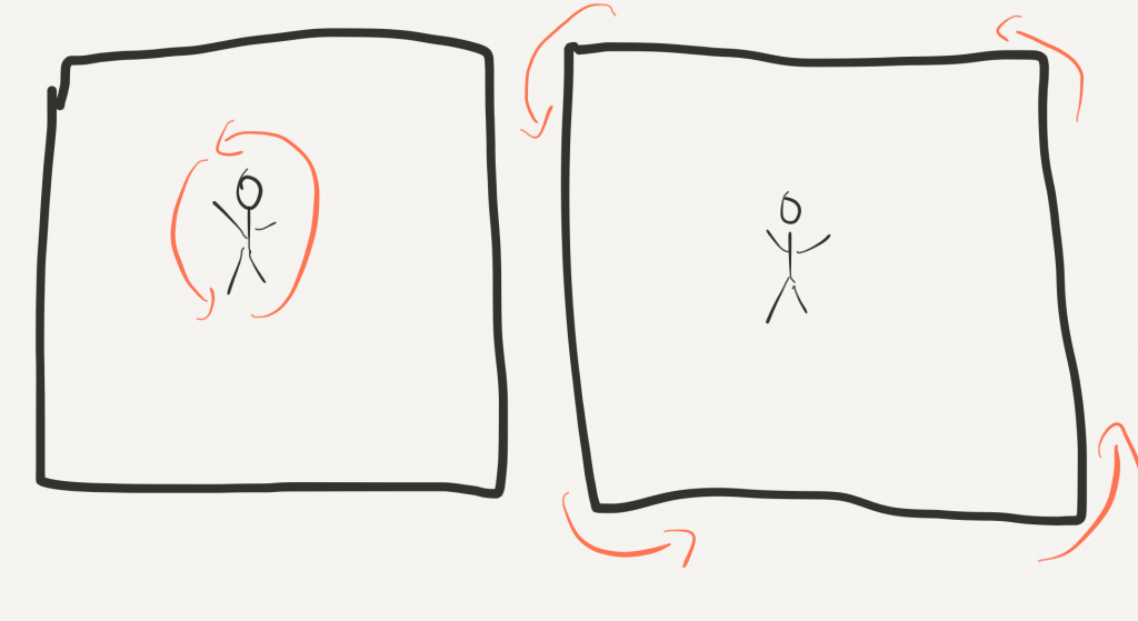
For example, let’s imagine an infinite, completely empty universe with just one observer somewhere inside. Is he stationary? What if he starts spinning? Would he feel dizzy? How could he tell that he spins at all? What if the universe starts spinning around him? Would he feel dizzy? is there any way to distinguish these scenarios?

There are only two answers. Either there is an absolute frame of reference, let’s call it “God’s frame”, or there is no way to distinguish these situations. While many people preferred for a long time the first possibility, the second one is Einstein’s perspective. He was a huge fan of the philosopher Ernst Mach, who argued using many thought experiments that the idea of absolute motion makes no sense.

In special relativity, what one observer calls a moving object, is an object at rest for another observer. There is no way to make an absolute statement of the form “this object is moving!”. In contrast, we can always state absolutely “this object is accelerating”.

However, Einstein’s hope was that it would be equally possible to make acceleration relative somehow. What one observer would call an accelerating object, another would call an object at rest. If this would be possible somehow, the laws of nature would be exactly the same for accelerating observers and observers at rest.

As already mentioned above, there are many good reasons to believe that this is simply not possible. Just take the next train and you’ll see how different accelerating frames are! Einstein was well aware of these obstacles, but he was obsessed by the idea that no frame should be special.

To move forward, we need to find out what makes accelerated frames special. Einstein, as any student of physics, learned in his mechanics lectures that in accelerating frames we need to take care of additional forces, called “fictitious forces”. These additional forces take care of the anomalous movement of objects in accelerating frames. A special feature of fictitious forces is that they are proportional to the mass of the object in question. While thousands of students learned these things every year, no one paid special attention to them. This is no wonder. Calculations in accelerated frames are extremely complicated and you can always simply choose another observer that isn’t accelerating.

However, Einstein was obsessed with his idea that no frame should be special and somehow at the right moment, these distant memories of what he learned in his mechanics’ course started popping up.

Another thing every student of physics learns is Newton’s formula $ m M /d^2$ that describes the gravitational force between two objects of mass $m$ and $M$ that are separated by a distance $d$. This law is completely analogous to Coulomb’s law $qQ/d^2$ that describes the electric force between two charged objects. The only difference is that gravity is always attractive, while the electric force can also be repelling. (Like charges repel each other, while unlike charges attract each other)

Remembering these two facts about accelerating frames and gravity, Einstein’s thought process could have been as follows:

“Fictitious forces are proportional to the mass of the object in question … The gravitational force is equally proportional to the mass of the object in question … Gravity reminds me of a fictitious force… Maybe gravity is a fictitious force!”

To explore this possibility, let’s imagine a spacetime somewhere in the universe far away from anything else. Usually, the astronauts in a spaceship float around of the spaceship aren’t accelerating. There is no way to call one of the walls the floor and another one the ceiling.

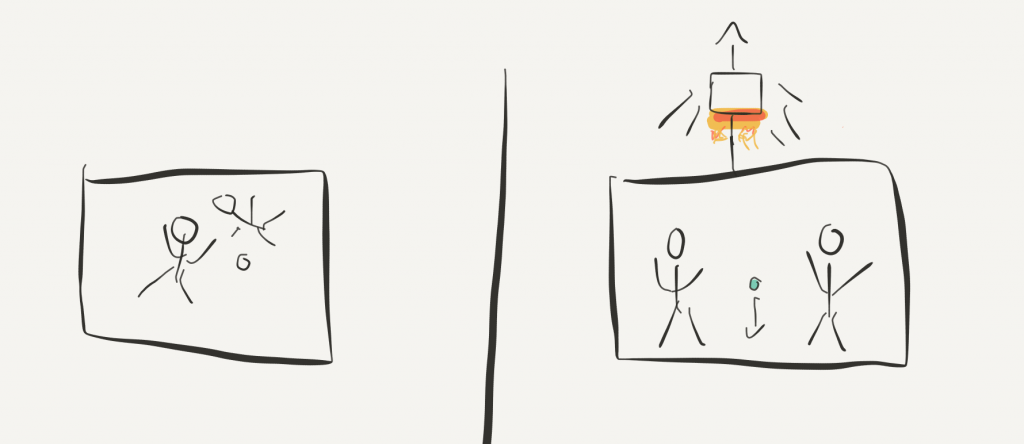
Now, what happens if another spaceship starts pulling the original spaceship? Immediately there is an “up” and a “down”. The passengers of the spaceship get pushed towards one of the walls. This wall suddenly becomes the floor of the spaceship. If one of the passengers drop an apple it falls to the floor.

For an outside observer, this isn’t surprising. Through the pulling of the second spaceship, the floor is moving towards the floating pencil. This leads to the illusion for the passengers inside the original spaceship that the pencil falls to the floor.

If there is no window in the original spaceship, there is no possibility for the astronauts to tell if they are sitting still on some planet or if they are accelerating. If their spaceship sits on a planet the pencil and the passengers themselves would be equally pulled to the floor, however in this case through gravity.

Even if we try to exploit some special possibility of gravity, there is no way to distinguish these situations. For example, a bowling ball and a pencil that is released from the same height would hit the floor at the same moment. This is what Galileo demonstrated for gravity, by throwing things down the Tower of Pisa. For an observer outside of the original spacetime, this fact would be by no means mysterious. The floor simply moves constantly towards the floating bowling ball and pencil. Hence, the floor touches the pencil and the bowling ball at exactly the same moment.

An outside observer would call the force that pushes thing to the floor in the original spacetime a fictitious force. It is merely a result of the floor moving towards the floating objects. However, for the passengers inside the spaceship, the force would be very real. They experience a real floor and a real ceiling and things really fall down if you let them drop. Without getting an outside view, it would be impossible for them to distinguish this fictitious force caused by the acceleration of their spaceship, from the force we call gravity. They can’t distinguish between acceleration and sitting at rest in an appropriate gravitational field.

This is crazy. Consider where we started. We were certain that accelerating frames are easily distinguishable. But now we find ourselves in a situation where we can’t find any difference between an accelerating frame and a stationary frame in a gravitational field.

Of course, the situation is only indistinguishable if the acceleration has a precise value that mimics the effect of the gravitational field. If you want to mimic the earth’s gravitational field, you need to accelerate quicker, than if you want to mimic the weaker gravitational field of the moon.

By remembering a simple fact about fictitious forces, Einstein was able to expand his principle of relativity even further. Now, even accelerating frames aren’t that special anymore.

This observation that accelerated frames are indistinguishable from a resting frame immersed in a gravitational field is called, well, the principle of equivalence.

The Principle of Equivalence

To bring this point really home, let’s imagine another situation. Instead of a spaceship somewhere in the middle of nowhere, let’s consider a spaceship floating 100 kilometers above the earth. The spaceship is pulled down by the earth’s gravitational field, but for the moment let’s imagine the spaceship is stationary. In this situation, the astronauts in the spaceship are able to distinguish “up” and “down” without problems. A pencil falls down, thanks to the earth’s gravitational field.

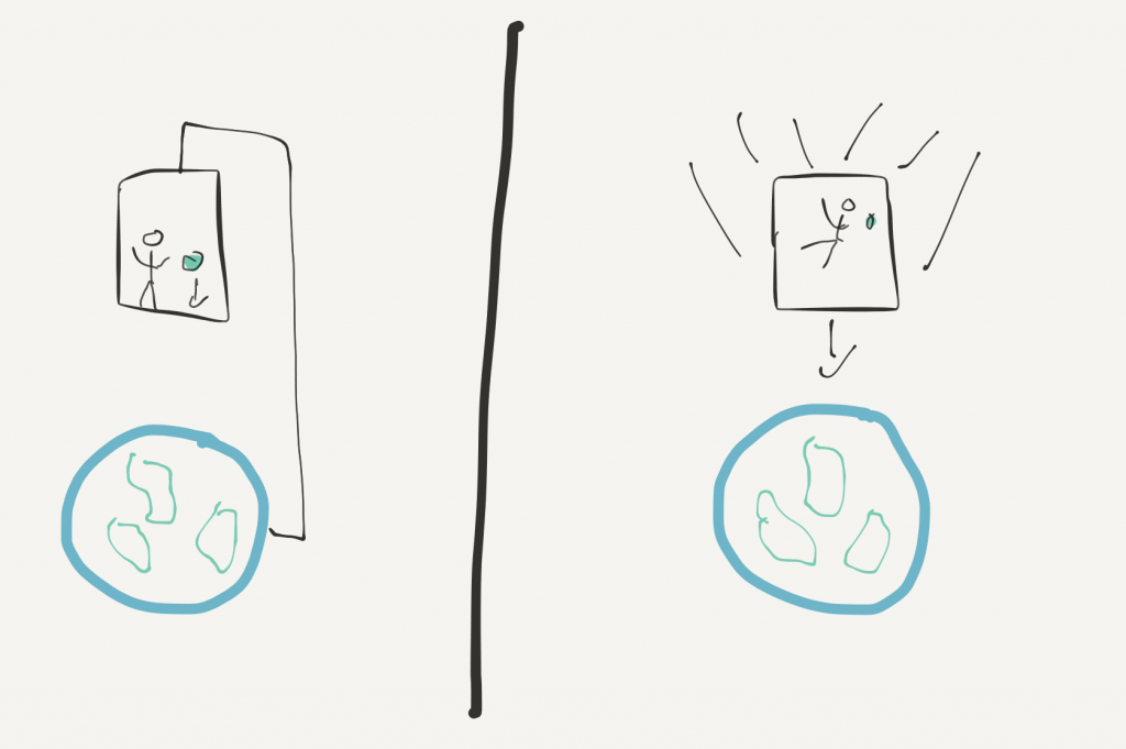
Then suddenly the spaceship is released from whatever holds it still 100 kilometers above the earth. What happens now? Of course, the spaceship starts falling down, i.e. moves towards the earth. At the same time the notions “up” and “down” start losing their meaning for the astronauts inside the spaceship. Everything inside the spaceship falls down towards the earth with exactly the same speed. This property of gravity was demonstrated by Galileo through his famous experiments at the Tower of Pisa. Thus, everything inside the spaceship starts floating. They experience zero gravity. For them, without the possibility to look outside of their spaceship, there is no gravitational field and nothing is falling down.

Therefore, gravity is nothing absolute. While for some observers there is a gravitational field, for the free-falling observers inside the spaceship there is none. If we want, we can therefore always consider some frame where there is no gravity at all! The gravitational force vanishes completely inside the free-falling spaceship. In contrast, an observer standing on earth would describe the spaceship by taking the earth’s gravitational field into account. To such an observer everything falls down because of this gravitational field. However, for the astronauts inside the spaceship, nothing is falling.

This situation is exactly the reversed situation to our first imaginary scenario. There we considered a spaceship somewhere in the middle of nowhere, where there was no gravitational field. Then the spaceship got pulled by another spaceship and suddenly the situation inside the original spaceship was as if they were immersed in a gravitational field. In our second imaginary situation, we started with a spaceship immersed in a gravitational field. However, all effects of this gravitational field vanish immediately when the spaceship starts falling freely towards the earth. Gravity has no absolute meaning. For some frames of reference there is gravity, for others, there isn’t.

The final Punchline

So far, we only considered linear acceleration. In both examples above the spaceship moved in a fixed direction with varying speed. However, not only when the magnitude of speed changes we have acceleration but also when an object changes direction. Another kind of accelerated frame is rotating frames.

The simplest kind of system we can consider is a disk that spins with a fixed number of revolutions per second. Each point on the disk undergoes a change in direction at every instant and is, therefore, accelerating all the time.

To understand a spinning disk we need to remember one of the most curious properties of special relativity: length contraction. The length of an object is smaller for some observer who moves with some velocity relative to the object than the length measured by some observer for whom the object is at rest.

Each point on our spinning disk moves round and round, but not in and out. Thus, according to special relativity, there is length contraction along the circumference, but none along the radius. Thus, when we measure the circumference of a spinning disk, we measure a different value than an observer who sits on the spinning disk. For the observer sitting on the spinning disk, the disk is at rest and hence no length contraction happens. However, we agree with this observer on the diameter of the disk, since even for us there is no radial movement of the disk.

The formula everyone learns in school for the relation of the radius $r$ to the circumference $C$ of a circle is:

$$ C = 2 \pi r . $$

Thus, the ratio of the circumference and radius that the observer on the disk, for whom the disk is at rest measures is $ C/r = 2 \pi$. For us outside observers, the disk spins and therefore there is length contraction along the circumference. Therefore, what we measure is not the same: $ C/r \neq 2 \pi$! This crazy result was known for some time as “Ehrenfest’s paradox”.

Once more Einstein understood what was going on here by remembering something he learned in a seminar. In a seminar about the geometry of two-dimensional curved surfaces, he learned that in non-Euclidean geometry the ratio $ C/r$ needs not necessarily be $2 \pi$. Depending on the surface we are considering the ratio can be any value.

The simplest example to understand this is a sphere. Let’s consider the ratio $C/r$ for the equator of a sphere, say the earth. The circumference is some number $C= C_E$. The radius of this circle is the distance from any point on the equator all the way up to the north pole. For a perfect sphere, the length of such a line is exactly one-half equator: $r= C_E /2$. Therefore, the ratio $C/r$ for a circle on a sphere is not $2 \pi$, but $C/r= C_E /(C_E / 2) = 2$!

Einstein remembered this property of curved surfaces and connected it with the seeming paradox situation concerning the $C/r$ ratio of a spinning disk. The mathematics of how to describe things on curved surfaces was at this time already developed by Gauss and Riemann. Einstein’s idea was to borrow these mathematical tools to describe what is going on in accelerating frames. Thanks to his equivalence principle accelerating frames are equivalent to resting frames in a gravitational field. Hence he noted that he could use the mathematics of Gauss and Riemann to describe gravity.

The Einstein Equation

Now, all we have to do is write down the correct equation that describes the idea “gravity = curved spacetime” mathematically. Einstein needed 6 years to discover the correct formula, but nowadays with the power of hindsight, the derivation is relatively straight-forward.

What causes gravity is mass, and thanks to Einstein’s famous formula $E = m c^2$, we know that equally energy causes gravity. Thus, at one side of our equation, we must have something describe the “charge” of gravity, i.e. energy. In mathematical terms, the “charge” of gravity is described by the energy-momentum tensor $ T_{\mu \nu}$.

As a first step towards our equation, we must now remember one of the most important laws of physics: the conservation of energy and momentum. In mathematical terms this conservation law is expressed as

\begin{equation} \partial^\mu T_{\mu \nu} = 0. \end{equation}

Next, we need something to describe curvature mathematically. This is what makes general relativity computationally very demanding. The most important object in this context is the metric. Metrics are mathematical objects that enable us to compute the distance between two points. In a curved space, the distance between two points is different than in a flat space as illustrated the following figure: (Geodesic)

Therefore metrics will play a very important role when thinking about curvature in mathematical terms.

Having talked about this, we are ready to “derive” the Einstein equation. It turns out that there is exactly one mathematical object that we can put on the left-hand side: the Einstein tensor $G_{\mu \nu}$. The Einstein tensor is the only divergence-free ($\partial^\mu G_{\mu \nu}=0$) function of the metric $g_{\mu\nu}$ and at most its first and second partial derivative. Therefore, the Einstein tensor may be very complicated, but it’s the only object we are allowed to write on the left-hand side describing curvature. This follows, because we can conclude from
\begin{equation} T_{\mu \nu} = C G_{\mu \nu} \quad \text{ that } \quad \partial^\mu T_{\mu \nu} = 0 \rightarrow \partial^\mu G_{\mu \nu} = 0\end{equation}
must hold, too. The Einstein tensor is a second rank tensor and has exactly this property. Second rank tensor means two indices $\mu \nu$, which is a necessary requirement, because $T_{\mu \nu}$ on the right-hand side has two indices, too.

The Einstein tensor is defined as a sum of the Ricci Tensor $R_{\mu\nu}$ and the trace of the Ricci tensor, called Ricci scalar $R =R_{\nu}^\nu$
\begin{equation} G_{\mu \nu} = R_{\mu\nu}-\frac{1}{2}Rg_{\mu \nu} \end{equation}
where the Ricci Tensor $R_{\mu\nu}$ is defined in terms of the Christoffel symbols $\Gamma^\mu_{\nu \rho}$

\begin{equation}
R_{\alpha\beta} = \partial_{\rho}{\Gamma^\rho_{\beta\alpha}} – \partial_{\beta}\Gamma^\rho_{\rho\alpha} + \Gamma^\rho_{\rho\lambda} \Gamma^\lambda_{\beta\alpha} – \Gamma^\rho_{\beta\lambda}\Gamma^\lambda_{\rho\alpha} \end{equation}
and the Christoffel Symbols are defined in terms of the metric
\begin{equation}
\Gamma_{\alpha \beta \rho} =\frac12 \left(\frac{\partial g_{\alpha \beta}}{\partial x^\rho} + \frac{\partial g_{\alpha \rho}}{\partial x^\beta} – \frac{\partial g_{\beta \rho}}{\partial x^\alpha} \right) = \frac12\, \left(\partial_{\rho}g_{\alpha \beta} + \partial_{\beta}g_{\alpha \rho} – \partial_{\alpha}g_{\beta \rho}\right). \end{equation}
This can be quite intimidating and shows why computations in general relativity very often need massive computational efforts.

Next, we need to know how things react to such a curved spacetime. What’s the path of an object from A to B in curved spacetime? The first guess is the correct one: An object follows the shortest path between two points in curved spacetime. We can start with a given distribution of energy and mass, which means some $T_{\mu \nu}$, compute the metric or Christoffel symbols with the Einstein equation and then get the trajectory through the \textbf{geodesic equation}
\begin{equation} \label{eq:geodesics}
\frac{d^2x^\lambda }{dt^2} + \Gamma^{\lambda}_{\mu \nu }\frac{dx^\mu }{dt}\frac{dx^\nu }{dt} = 0.
\end{equation}
The geodesic is the locally shortest curve between two points on a manifold. (This is a bit oversimplified, but the correct definition needs some terms from differential geometry we haven’t introduced here.)

That’s it.

My plan is to write next about why this idea “gravity = curvature” is not the really the essence of general relativity. This somewhat controversial statement is something that even Einstein himself only understood after several decades. However, this post is already incredibly long and thus I’ll write another post about this.

To finish this post, here are some recommendations where to read more about Einstein’s theory: 

My favorite GR textbooks are


A Mystery called Wick Rotation or can we understand the “Action” Formalism?

The Wick rotation pops up as a “mere technical trick” in quantum field theoretical calculations. Making the time coordinate complex $t \to i \tau$ is described as “analytic continuation” and helps to solve integrals. Certainly, there is nothing deep behind this technical trick, right?

Well, I’m no longer so sure.

There is one observation that makes me (and others) wonder:

The difference between the mystical theory of quantum fields and ordinary statistical mechanics is a Wick rotation $ t ➝ i /(kT) $.

This is puzzling. On the one hand, we have ordinary statistical mechanics that we understand perfectly well. When we want to make a statement about a system where we don’t know all the details, we invoke the principle of maximum entropy and get as a result the famous Boltzmann distribution $\propto exp(-E/T)$. This distribution tells us the probabilities to find the system, depending on the energy $E$, in the various macroscopic states. There is nothing mysterious about this. The principle of maximum entropy is simply an optimal guessing strategy in situations where we don’t know all the details. (If you don’t know this perspective on entropy you can read about it, for example, here). This interpretation due to Jaynes and the derivation of the Boltzmann distribution are completely satisfactory. It is no exaggeration when we say that we understand statistical mechanics.

On the other hand, we have the mysterious “probability distribution” in quantum field theory that is known as the path integral. I know no one who claims to understand why it works. The path integral is proportional to $exp(iS/\hbar)$, where $S$ denotes the action and even Feynman admitted:

I don’t know what action is“.

In his book QED, when he talks about the path integral, he writes

Will you understand what I’m going to tell you? …No, you’re not going to be able to understand it. … I don’t understand it. Nobody does.

It seems as if all the mysteries of the quantum world are encapsulated in a simple Wick rotation.

I’ve been searching for quite a while but wasn’t able to find any sufficient discussion of this curious fact.

There was some “recent” work by John Baez, which he described in his blog and also a paper. He also tried to make sense of Wick rotations by making use of it in a classical mechanics example. (See the “Homework on A spring in imaginary time” here and additionally, the discussion here). The lesson there was that “replacing time by “imaginary time” in Lagrangian mechanics turns dynamics problems involving a point particle into statics problems involving a spring.” In addition, several years ago Peter Woit tried to emphasize the confusion surrounding Wick rotations in a blog post. He wrote:

“I’ve always thought this whole confusion is an important clue that there is something about the relation of QFT and geometry that we don’t understand. Things are even more confusing than just worrying about Minkowski vs. Euclidean metrics. To define spinors, we need not just a metric, but a spin connection. In Minkowski space this is a connection on a Spin(3,1)=SL(2,C) bundle, in Euclidean space on a Spin(4)=SU(2)xSU(2) bundle, and these are quite different things, with associated spinor fields with quite different properties. So the whole “Wick Rotation” question is very confusing even in flat space-time when one is dealing with spinors.”

However, apart from that, there don’t seem to be any good discussions of the “meaning” of a Wick rotation and I still don’t know what to make of it. Yet, it seems clear that something very deep must be going on here. If the Boltzmann distribution can be understood perfectly by invoking the “best guess” strategy known as “maximal entropy”, has the path integral a similar origin? Probably, but so far, no one was able to find it.

In statistical mechanics, our best guess for the macroscopic state our system is in the state that can be realized through the maximal number of microscopic states. This state is known as the state with maximal entropy. Many microscopic details make no difference for the macroscopic properties and therefore, many microscopic configurations lead to the same macroscopic state. We don’t know all the microscopic details but want to make a statement about the macroscopic properties. Hence, we must use the best guess approach, and the best guess is the macroscopic state with maximum entropy.

Aren’t we doing in quantum theory something similar? We admit that we don’t know the fundamental microscopic dynamics. We don’t know which path a given particle takes from point $A$ to point $B$. Nevertheless, when pressured, we make a guess. Our best guess is the path with extremal action.

The observation by John Baez mentioned above that a Wick rotation connects a static description, like in statistical mechanics, with a dynamical description, like in quantum field theory, seems to make sense from this perspective.

Some nice thoughts in this direction are collected by Tommaso Toffoli in his two papers: “What Is the Lagrangian Counting?” and “Action, Or the Fungibility of Computation“. For example, he writes:

just as entropy measures, on a log scale, the number of possible microscopic states consistent with a given macroscopic description, so I argue that action measures, again on a log scale, the number of possible microscopic laws consistent with a given macroscopic behaviour. If entropy measures in how many different states you could be in detail and still be substantially the same, then action measures how many different recipes you could follow in detail and still behave substantially the same.

In addition, I think there could be a connection to recent attempts to understand quantum theory as extended probability theory, where we allow negative probabilities. This line of thought leads to complex probability amplitudes like we know them from quantum theory. For a nice introduction to this perspective on quantum theory, see this lecture by Scott Aaronson. Interestingly he argues that this extension of probability theory is all we need to derive quantum theory. Again, the switch to complex quantities seems to make all the difference.

I think this is a good example of an obvious, but, so far, not sufficiently understood the connection that could yield deep insights into the quantum world. I usually write about things, where I think I have understood something. However, here I mainly wrote this to organize my thoughts and as a reminder to think more about this in the future.

To finish, here is an incomplete list, where Wick rotations are also crucial

1.) We use a Wick rotation to classify all irreducible representations of the Lorentz group. In this context, the Wick rotation is often called “Weyl’s unitary trick”.
2.) A Wick rotation is used to analyze tunneling phenomena, like, for example, the famous instanton solutions in QFT.
3.) People who consider QFT at finite temperatures make heavy use of Wick rotations.

Demystifying the QCD Vacuum – Part 5: Anomalies and the Strong CP Problem

There is a deep connection between the non-trivial structure of the QCD vacuum and one of the most mysterious phenomenon in QFT: anomalies. In this part, we discuss this connection.

The thing is that, so far, we only talked about the vacuum of the gauge bosons, without saying a word about fermions. We will now see that the fermionic vacuum isn’t trivial either and that there is a close connection to what we discussed earlier for the pure gauge vacuum.

The Chiral and Axial Symmetry

If we take a look at the QCD Lagrangian with, for simplicity, just one massless quark:

$$ \mathcal{L} = -\frac{1}{4}G_a^{\mu\nu} G_{a\mu\nu} + \bar{\Psi} (i\partial_\mu \gamma^\mu -g A_\mu \gamma^\mu ) \Psi$$

we notice that there is a global symmetry

$$ \Psi \to e^{i\varphi} \Psi . $$

The conserved charge that belongs this symmetry via Noether’s theorem is simply the number of $\Psi$ particles. However, there is even more symmetry.

We can rewrite the Lagrangian in terms of left-chiral and right-chiral spinors, with the help of the usual projection operators: $\Psi_{L/R}= \frac{1}{2} (1 \pm\gamma_5) \Psi$. Then, we have

$$ \mathcal{L} = -\frac{1}{4}G_a^{\mu\nu} G_{a\mu\nu} + \bar{\Psi}_L (i\partial_\mu \gamma^\mu-e A_\mu \gamma^\mu ) \Psi_L + \bar{\Psi}_R (i\partial_\mu \gamma^\mu -eA_\mu \gamma^\mu) \Psi_R $$

and we can see that we actually have here two global symmetry:

\begin{align}
\Psi_L \to e^{i\alpha} \Psi_L \notag \\
\Psi_R \to e^{i\beta} \Psi_R
\end{align}

The corresponding Noether charges tell us that the number of left-chiral and right-chiral particles are conserved separately!

We can multiply the right-chiral and left-chiral spinors by completely different phases because there is no term here that couples left-chiral to right-chiral spinors. (Take note that a mass term couples left-chiral to right-chiral spinors and we discuss the implications of mass terms later).

At this point, you may wonder, why we care about symmetries in such an unrealistic situation. Every quark is massive and therefore we don’t actually have these symmetries! However, the masses of the two lightest quarks, the up and down quark are so tiny that they can be neglected without making a too large error. In this sense, symmetries that are present in the absence of the masses of the lightest quarks are good approximate symmetries. Such approximate symmetries are often very useful to learn something. For example, if we neglect the masses of the up quark and the down quark, we have an $SU(2)$ symmetry. This symmetry gets broken, but only a little, by the small actual masses of the up quark and the down quark. This small breaking tells us that we can expect Goldstone bosons that correspond to this breaking. Of course, because the symmetry is only an approximate one, we don’t get real massless Goldstone bosons. Yet, we get quasi-Goldstone bosons, called pions, and the approximate symmetry perspective explains why they are so light compared to all other mesons.

However, our motivation here is a bit different. Namely, we will see in a moment that even in the absence of quark masses, which would break one linear combination of these symmetries, one linear combination is broken! This anomalous breaking of the symmetries has an important implication that can actually be measured in experiments.

Now, back to our symmetries.

Noether’s theorem tells us that to each symmetry, we get a conserved current. The conserved currents here are

\begin{align}
J_L^\mu = \Psi_L \gamma_\mu \Psi_L \notag \\
J_R^\mu = \Psi_R \gamma_\mu \Psi_R
\end{align}

However, upon closer inspection, which will be discussed in a moment, it turns out that these separate currents are not conserved at all. Yet, we can find a linear combination that is conserved:

\begin{align}
J_V^\mu = J_L^\mu + J_R^\mu =\bar{\Psi} \gamma_\mu \Psi \notag \\
\partial_\mu J_V^\mu =0.
\end{align}

In turn, the orthogonal linear combination is not conserved:

\begin{align}
J_A^\mu = J_L^\mu – J_R^\mu =\bar{\Psi} \gamma_\mu \gamma_5 \Psi \notag \\
\partial_\mu J_A^\mu \neq 0.
\end{align}

The symmetry that corresponds to the conservation of $J_V^\mu$ is known as “vector $U(1)$” and denoted by $U(1)_V$. An $U(1)_V$ transformation is given by

$$ \Psi \to e^{i\phi_v} \Psi . $$

The symmetry that would exist if $J_A^\mu$ would be conserved, is known as “axial $U(1)$” and denoted by $U(1)_A$. An $U(1)_A$ transformation is given by

$$ \Psi \to e^{i \phi_a \gamma_5} \Psi . $$

The connection to the previous transformations that acted on $\Psi_L$ and $\Psi_R$ is given by $\alpha = \phi_v+\phi_a$ and $\beta = \phi_v-\phi_a$.

The situation here is similar to what happens in the standard model. There $SU(2)_L \times U(1)_Y$ gets broken to $U(1)_{em}$. The thing is that $U(1)_{em}$ is not $U(1)_Y$, but a linear combination of $U(1)_Y$ and the Cartan generator of $SU(2)_L$. Here we start with $U(1)_L \times U(1)_R$, and this symmetry “gets broken” to $U(1)_V$.

How does $U(1)_A$ get broken?

Above, we only stated that $U(1)_A$ gets broken. However, that this breaking happens is far from obvious. There is no scalar field in the theory that could be responsible for the breaking. Instead, we are dealing here with a more subtle type of symmetry breaking, called quantum mechanical symmetry breaking. A symmetry that is present in the classical theory, i.e. when we simply look at the Lagrangian, is no symmetry as soon as we use the Lagrangian in a quantum theory.

The conventional name for such quantum mechanical symmetry breaking is “anomalous breaking”.

There are several ways to see that this anomalous breaking happens.

Historically this was first discovered through a quite complicated computation of a Feynman diagram called “triangle diagram”.

The result of this computation by Adler, Bell, and Jackiw was

$$ \partial_\mu J_5^\mu = \frac{g^2}{16\pi^2} G^{\mu\nu a} \tilde{G}_{\mu \nu}^a $$

This looks shockingly like the term that we added to the Lagrangian due to the complex structure of the QCD vacuum. (This was discussed in part 4). The details regarding this laborious computation can be found in the standard textbooks, but aren’t very illuminating. Thus, we won’t go into the details here.

Instead, I want to focus on the implications and a more illustrative explanation.

Understanding the Axial Anomaly

To understand the axial anomaly, we consider the vacuum in a theory of massless fermions. To understand the theory and its vacuum, we consider its energy levels. In practice this means, we calculate the eigenmodes of the Hamiltonian.

The best picture of this vacuum is Dirac’s “sea picture”. All states with negative energy a filled up, whereas all positive energy states are empty. An electron is a positive energy state, whereas a positron is a hole in the sea of negative energy states.

In the real world, however, fermions are never alone because they carry charges. Thus, we now investigate what happens when we take the presence of gauge fields into account. We will then see that the axial anomaly is nothing but a natural consequence of the interplay between the Dirac sea and gauge fields.

To simplify the discussion, we work in two dimensions and use electromagnetic interactions, instead of the more complicated QCD interactions. The massless theory of fermions in two-dimensions, with only electromagnetic interactions present, is known as the Schwinger model. The Schwinger model is incredibly useful to understand many phenomena in quantum field theory and will prove to be invaluable here.

To simplify the discussion even further, we work in the temporal gauge: $A_0=0$. This means our gauge field has only one component $A_1 \equiv A$.

In our two-dimensional theory, we split our spinor again depending on their chirality:

$$ \Psi_+ = \begin{pmatrix} 1 & 0 \\ 0 &0 \end{pmatrix} \Psi $$
$$ \Psi_- = \begin{pmatrix} 0 & 0 \\ 0 &1 \end{pmatrix} \Psi $$

Particles with positive “chirality” are here simply particles that move to the left on our one-dimensional spatial axes (the second dimension is the time axes.) Formulated differently, positive “chirality” states are states with negative momentum. Equivalently, negative “chirality” states are states that move to the right and therefore have positive momentum.

Completely analogous to our four-dimensional problem, we can find here an anomalous divergence. Here it is proportional to $\epsilon^{\mu\nu} F_{\mu\nu} \propto \partial_t A$. We now want to answer the question: What is the origin of this anomalous divergence?

The Dirac equation for our two-dimensional model reads

$$ H \Psi_E = -\sigma_3 (\hat p – g A) \Psi_E = E\Psi_E. $$

The energy eigenstates are

\begin{align}
\Psi_+ &= \begin{pmatrix} e^{ipx} \\0 \end{pmatrix} \text{ with energy } E=-p+qA \notag \\
\Psi_- &= \begin{pmatrix} 0 \\ e^{ipx} \end{pmatrix} \text{ with energy } E=p-qA
\end{align}

Now, in the absence of the gauge field $A$, we have for the vacuum the simple Dirac sea picture outlined above. All the negative energy states are filled, while all the positive energy states are empty.

However, something interesting happens when we switch on the gauge field. As the magnitude of $A$ increases from $0$ to $\delta A$, we can see how the energy levels shift. This is best explained by a picture:

Source: https://arxiv.org/pdf/hep-th/9903255.pdf

The states with positive chirality, and hence negative momentum, do have a higher energy thanks to the gauge field $A$. In contrast, the energy levels of states with negative chirality (= positive momentum) get lower when we switch on $A$.

For the Dirac sea, this means that states that were once negative energy states and therefore filled states become now filled positive energy states. Equivalently unfilled positive energy states (= holes) now have negative energy and move below the zero energy border. In other words, the gauge field produces holes in the negative energy sea and filled positive energy states.

Let’s consider, for concreteness a positive magnitude of the gauge field $A = \delta A > 0$:

An empty state with positive momentum, positive energy, and left chirality, now acquires negative energy and therefore becomes a right-chiral antiparticle.

A filled state with negative momentum, negative energy, and right-chirality, now acquires positive energy and therefore becomes a left-chiral particle.

This means immediately that in the presence of a gauge field $A$ the charge “left-chirality” and the charge “right-chirality” are not conserved. However, the sum of “left-chirality” and “right-chirality” is still conserved! This is analogous to what we observed for the conserved current $J_L^\mu$ and $J_R^\mu$.

This is the origin of the anomaly! The gauge field produces a non-zero chirality current by lifting some states up from the Dirac sea and by pushing some holes down into the negative energy region.

It is important to take note that the shift from $A=0$ to $A= \delta A$ is a gauge transformation! The crazy thing that happens here is that such gauge transformation produces particles from the empty vacuum and this is why we get a non-zero current. What we learn here is that it is impossible to separate left-chiral and right-chiral states in a gauge invariant manner.

The fermionic vacuum, i.e. the Dirac sea, is highly susceptible to the gauge field configurations. The mere presence of the gauge fields changes the structure of the energy eigenstates and hence of the Dirac sea dramatically.

As an aside, that will be discussed in more detail in another post: This type of fermion production through gauge fields is the most popular explanation for why there is any matter at all. This explanation is known as Leptogenesis and the main idea is that topological non-trivial gauge field changes can be responsible for a nett baryon number plus lepton number surplus, while baryon minus lepton number remains unchanged.

Another important lesson here, to quote Roman Jackiw, is that:

“we must assign physical reality to Dirac’s negative energy sea, because it produces the chiral anomaly, whose effects are experimentally observed, principally in the decay of the neutral pion to two photons, but there are other physical consequences as well.”

Now, what does this mean for our axial anomaly in four dimensions?

We know that the axial current $J_5^\mu$ is anomalously non-conserved. This means that the divergence $\partial_\mu J_5^\mu$ is non-zero, and a calculation shows that it is $\propto Tr( F_{\mu\nu} \tilde{F}^{\mu\nu})$. Thus, the corresponding Noether charge

$$ Q = \int d^3 x J^0_5 $$

is not conserved. Especially, in any process where the gauge fields change such that

$$ N = \frac{1}{32 \pi^2} \int d^4x Tr( F_{\mu\nu} \tilde{F}^{\mu\nu}) \neq 0 , $$

the Noether charge $Q$ gets changed. Such a process was already discussed in the first three parts, and are commonly known as instanton and sphaleron processes. These processes change the winding number $N$. Thanks to the connection to the axial anomaly that we know now of, we understand that such processes produce a nett surplus of left-chiral and right-chiral states. Yet, the number of left-chiral minus the number of right-chiral states remains unchanged. The quantum number “left-chirality” plus “right-chirality” is not conserved and this is the breaking of the axial symmetry.

Topologically non-trivial processes like instantons and sphalerons lift fermions up from the Dirac sea and push unfilled positive states down to negative energies. This way, instantons, and sphalerons produce fermions and anti-fermion pairs.

To quote from Eric Weinberg’s book “Classical Solutions in Quantum Field Theory“:

“any change in winding number must be accompanied by a change in fermion chirality”

If you interested to learn more about this perspective on anomalies, here are a few good resources, where you can learn more:

Implications of the Axial Anomaly

So, the non-conservation of the axial current $ \partial_\mu J_5^\mu \neq 0$ tells us that axial rotations $ \Psi \to e^{i \phi_a \gamma_5} \Psi $ are not a symmetry of the system. Therefore, we can now ask: How does the Lagrangian change under axial rotations?

As for anything that has to do with anomalies, there are many ways to answer this question. But, of course, the final answer is always the same:

An axial rotation $ \Psi \to e^{i \phi_a \gamma_5} \Psi $ changes our Lagrangian by

$$ \mathcal{L} \to \mathcal{L} + \frac{\alpha}{16 \pi^2} Tr[G_{\mu\nu} \tilde{G}^{\mu\nu}] . $$

Compare this to the term that we needed to add, because of the complex structure of the QCD vacuum:

$$\Delta \mathcal L = \frac{\theta}{16 \pi^2} Tr[G_{\mu\nu} \tilde{G}^{\mu\nu}]$$

It’s exactly the same!

Thus, we can say that an axial rotation by $\alpha$ shifts the mysterious $\theta$ parameter of the QCD vacuum by:

$$ \theta \to \theta + \alpha .$$

So, why does an axial rotation lead to this new term in the Lagrangian? As already mentioned above, there are different ways to see this.

1.) The standard method that is usually quoted in the textbook is known as “Fujikawa method”. (It has its own Wikipedia page). Again, I don’t want to dive into the technical details, which you can find in the standard textbooks. However, the short version is that once careful analyzes the behavior of the path integral under an axial rotation. While the Lagrangian behaves, of course, as expected from the discussion above and stays unchanged, the measure of the path integral isn’t invariant. Instead, the final result of Fujikawa’s analysis is that the change in the path integral measure due to an axial rotation amounts exactly to the change

$$ \mathcal{L} \to \mathcal{L} + \frac{\alpha}{16 \pi^2} Tr[G_{\mu\nu} \tilde{G}^{\mu\nu}] . $$

of the Lagrangian.

2.) Another way to see this is to go directly back to Noether’s theorem. (See
Palash Pal’s “An Introductory Course of Particle Physics” Eq. 4.108 at page 82 plus page 658 Eq. 21.158 or page 250 in “Classical Solutions in Quantum Field Theory” by Erick Weinberg, especially Eq. 11.57 and the text below.)

In the derivation of this theorem in the Lagrangian formalism, we calculate that when a field gets transformed

$$ \Psi^A(x) \to \Psi’^A(x)=\Psi^A(x) + \delta \Psi^A(x), $$

the change of the action is

$$ \delta S = \int d^4 x \sum_r \delta \varphi_r \partial_\mu J_r^\mu, $$

where

$$ J_r = \sum_A \frac{\partial\mathcal{L}}{\partial(\partial_\mu\Psi^A)} \frac{\partial\Psi^A}{\partial \varphi_r}$$

and  $\varphi_r$ denotes a small change in a number of parameters.

(This is shown, for example at page 106 and 107 in my book “Physics from Symmetry”. In addition, take note that, as usual in the derivation of Noether’s theorem, we only consider infinitesimal transformations).

If we are dealing with a symmetry, the action does not change: $\delta S =0$ and thus we have $ \partial_\mu J_r^\mu =0$, i.e. a conserved current.

However, here we have situation where we found that $ \partial_\mu J_A^\mu \neq 0$. Thus, the corresponding transformation,an axial rotation $ \Psi \to e^{i \varphi \gamma_5} \Psi $, is not a symmetry. We can therefore conclude that the action changes under such a rotation, and the change of the action is given by

$$ \delta S = \int d^4 x \sum_R \delta \varphi_r \partial_\mu J_r^\mu . $$

In our case,
$$ \partial_\mu J_5^\mu = \frac{g^2}{16\pi^2} Tr(G^{\mu\nu a} \tilde{G}_{\mu \nu}^a )$$

and therefore, the the action changes by

$$ \delta S = \int d^4 x \, \varphi \partial_\mu J_r^\mu = \frac{g^2 \varphi }{16\pi^2} \int d^4 x \, G^{\mu\nu a} \tilde{G}_{\mu \nu}^a . $$

3.) A third method to see this change of the action, is the original method by Jackiw and Rebbi (PhysRevLett.37.172). Again, we only discuss the main idea, and do not dive into the details.

The basic idea is the following: Instead of the non-conserved current $J_5^\mu$, we define a new current that is conserved. The corresponding Noether charge generates the corresponding symmetry. Then we investigate the how this Noether charge acts on our ground state $|\theta\rangle$. The result is the same as for the previous two methods:

$$ e^{i \alpha Q_5} |\theta\rangle = |\theta + \alpha \rangle.$$

So, now let’s see how this comes about in a bit more detail.

From the discussion above, we know that $J_5^\mu = \bar{\Psi} \gamma_\mu \gamma_5 \Psi $ is not conserved. Instead, we have

$$ \partial_\mu J_5^\mu = \frac{g^2}{16\pi^2} Tr(G^{\mu\nu a} \tilde{G}_{\mu \nu}^a) . $$

Now, an important observation is, that $G^{\mu\nu a} \tilde{G}_{\mu \nu}^a$ can be written as total divergence:

$$ \frac{1}{4} G^{\mu\nu a} \tilde{G}_{\mu \nu}^a = \partial_\mu K^\mu, $$

where

$$ K^\mu = \epsilon^{\mu \alpha\beta \gamma} Tr(\frac{1}{2} A-\alpha \partial_\beta A_\gamma + \frac{i}{3} g A-\alpha A_\beta A_\gamma) $$

(A proof of this statement can be found, for example at page 89 in “Quarks, Leptons and Gauge Fields by K. Huang.)

$K_\mu$ is commonly called the Chern-Simons term or Chern-Simons current.

With the observation that $ G^{\mu\nu a} \tilde{G}_{\mu \nu}^a$ can be written as total divergence, we can define a new, actually conserved, axial current:

$$ \tilde{J}_5^\mu = J_5^\mu – \frac{g^2}{16\pi^2} K^\mu . $$

The trick here is, of course, that if we not take the divergence of this new current, the two terms simply cancel:

$$ \partial_\mu \tilde{J}_5^\mu = \partial_\mu J_5^\mu – \partial_\mu \frac{g^2}{16\pi^2} K^\mu $$
$$= \frac{g^2}{16\pi^2} Tr(G^{\mu\nu a} \tilde{G}_{\mu \nu}^a) – \frac{g^2}{16\pi^2} Tr(G^{\mu\nu a} \tilde{G}_{\mu \nu}^a) =0 . $$

The generator $Q_5$ of this $\tilde{U}(1)_A$ is, as always, the corresponding Noether charge

$$ Q_5 \equiv \int d^3x J_5^0 = \int d^3x \left[\Psi^\dagger \gamma_5 \Psi – \frac{g^2}{16\pi^2} K^0 \right]. $$

A curious feature of this Noether charge is that it isn’t gauge invariant and therefore not a physical quantity. The reason for this is that $K^\mu$ isn’t gauge invariant.

Nevertheless, we have here the generator of a symmetry and we are now interested in how the $\theta$ vacuum, that we discussed in part 4, behaves under the transformation that is generated by $Q_5$.

To do this, we employ a trick. We already saw in part 4 that if we act with some gauge transformation with winding number $n$ on our vacuum state $|\theta\rangle$, we get $ g_n |\theta\rangle = e^{in \theta}$. The idea is now, to use this to find out if $\theta$ gets changed by $Q_5$. In other words, we want to compute

$$ g_n \left( e^{i\alpha Q_5} |\theta\rangle \right) = e^{i\theta’}\left( e^{i\alpha Q_5} |\theta\rangle \right) . $$

The resulting $\theta’$ tells us how $\theta$ is affected by $e^{i\alpha Q_5}$.

To compute this, we need to know how $Q_5$ changes under gauge transformations. The result is (see Jackiw and Rebbi 1976)

$$g_n Q_5 g_n^{-1} = Q_5 + 1 .$$

With this information at hand, we can calculate

\begin{align}
g_1 \left( e^{i\alpha Q_5} |\theta\rangle \right) &= g_1 e^{i\alpha Q_5} |\theta\rangle g_1^{-1} g_1\notag \\
&= e^{i\alpha (Q_5+1)}g_1\notag \\
&= e^{i\alpha (Q_5+1)} e^{i\theta} |\theta\rangle \notag \\
&= e^{i(\theta+ \alpha)} \left( e^{i\alpha Q_5} |\theta\rangle \right) \notag \\
&\equiv e^{i\theta’} \left( e^{i\alpha Q_5} |\theta\rangle \right)
\end{align}

and thus we can conclude

$$ e^{i\alpha Q_5} |\theta\rangle = |\theta + \alpha \rangle .$$

From the discussion in part 4 we know that the existence of the non-trivial ground state $|\theta\rangle$ implies a new term in the Lagrangian

$\Delta \mathcal L = \frac{\theta}{16 \pi^2} Tr[G_{\mu\nu} \tilde{G}^{\mu\nu}].$$

The observation here that $Q_5$ shifts $\theta$, then means that the $\theta$ that appears in this new term, get shifted. Hence, we are again led to the conclusion that a chiral rotation implies a new term in the Lagrangian

$$ \Delta \mathcal L = \frac{g^2 \alpha }{16\pi^2} G^{\mu\nu a} \tilde{G}_{\mu \nu}^a$$

The Strong CP Problem

We saw in the last section that an axial rotation by $\alpha$ shifts the $\theta$ parameter of the QCD vacuum by:

$$ \theta \to \theta + \alpha .$$

Without mass terms, we can define a conserved but non-gauge invariant axial symmetry. Then we can make use of this symmetry to get rid of the parameter $\theta$. We are free to do any rotation we want and therefore, we can easily rotate $\theta$ to zero.

However, if there are mass terms

$$ m \bar \Psi \Psi = m \bar{\Psi}_L \Psi_R + m \bar{\Psi}_R \Psi_L $$

for the quarks, we no longer have this freedom. The axial symmetry is broken explicitly by the mass terms, because we are no longer free to rotate the left-chiral spinors and right-chiral spinors independently. A mass term explicitly couples a right-chiral to a left-chiral spinor. Therefore, the only allowed transformation is now

\begin{align}
\Psi_L \to e^{i\alpha} \Psi_L \notag \\
\Psi_R \to e^{i\alpha} \Psi_R
\end{align}

and

\begin{align}
\Psi_L \to e^{i\alpha} \Psi_L \notag \\
\Psi_R \to e^{-i\alpha} \Psi_R
\end{align}

is no longer a symmetry. Transforming the left-chiral and the right-chiral spinor with the same phase is a $U(1)_V$ transformation, whereas a transformation with opposite phase is an $U(1)_A$ transformation. In this sense, we can say that mass term breaks $U(1)_A$ explicitly.

Yet, we are forced to perform an axial rotation. This comes about because, in order to understand the physical content of the theory, we like to work in the mass basis where the mass matrices are real and diagonal. In general, the mass matrices aren’t real and diagonal but instead contain complex entries. The transformation

\begin{align}
\Psi_L \to U_L\Psi_L \notag \\
\Psi_R \to U_R \Psi_R,
\end{align}

where $U_L$ are unitary matrices, that make the mass matrix real and diagonal (we suppress generational indices here) leads to the emergence of the CKM matrix in the gauge sector of the theory.

A crucial observation is now that this rotation that we perform to switch to the mass basis, in general, involves an axial rotation. In particular, the desired transformation involves the rotation

\begin{align}
\Psi_L \to e^{-i ArgDet(M)} \Psi_L \notag \\
\Psi_R \to e^{i ArgDet(M)} \Psi_R .
\end{align}

(See, Eq. 191 in https://arxiv.org/pdf/hep-ph/9807516.pdf)

Thus, in contrast to the discussion of a massless theory, we are here no longer free to perform arbitrary axial rotations. Instead, there is one very special axial rotation, by the angle $\alpha = ArgDet(M)$ that we need to make the mass matrix $M$ real and diagonal.

From the discussion in the last section, we know that an axial rotation by angle $\alpha$ changes the Lagrangian

$$ \mathcal L \to \mathcal L + \frac{g^2 \alpha }{16\pi^2} G^{\mu\nu a} \tilde{G}_{\mu \nu}^a . $$

If there are mass terms, the angle $\alpha$ is fixed and given by $\alpha = ArgDet(M)$.

Thus, on the one hand, we have a parameter $\theta$ that comes from the detailed study of the QCD vacuum. On the other hand, we have a shift of this parameter through an axial rotation of quark fields by the angle $\alpha = ArgDet(M)$.

To take these two observations into account, one usually introduces a new overall parameters

$$ \bar{\theta} = \theta + ArgDet(M). $$

From experiments we know, as mentioned at the end of part 4, that $\bar{\theta}$ is tiny: $ \bar{\theta} \lesssim 10^{-9} $. Thus, in some sense the two contributions to $\bar{\theta}$ must cancel very, very precisely. This is usually called a “fine-tuning” problem, because the QCD vacuum angle $\theta$ and the $ArgDet$ must be fine-tuned to extremely high precision to yield such a tiny overall $\bar{\theta}$.

This is often presented as a big mystery. Why should there be a connection between these two seemingly completely unrelated parameters? The parameter $\theta$ was discovered by studying the pure gauge vacuum. The shift of $\theta$ by the angle $alpha$ comes from the axial rotation of fermionic fields and has its deep origin in the axial anomaly.

However, from the discussion above it should be clear that these two contributions aren’t so unrelated after all. Both originate in non-perturbative processes like instantons.

The emergence of $\theta$ as a parameter that describes the QCD vacuum structure, was a result of instanton process. In the temporal gauge, we discovered

An unrealistic solution of the strong CP problem

One trivial solution to the strong CP problem was, in principle, already mentioned above. Without a mass term $\bar{\theta}$ wouldn’t be a physical parameter because we can give it any term we want through axial rotations. However, if there is a mass term, we no longer have this freedom.

In the real world, there are many quarks and therefore, in the absence of mass terms many axial symmetries: one for each quark. This means immediately that when one quark is massless, say the up-quark, we could perform an arbitrary axial rotation of the corresponding spinors. Following the discussion above, this would immediately mean that $\theta$ is not a physical quantity because we can change it at will via this axial rotation.

Only, if all fermions do have mass, $\bar{\theta}$ is a physical parameter. However, as far as we know this is actually the case and therefore $\bar{\theta}$ physical. Yet, “one massless quark” is commonly quoted as a solution of the strong CP problem.